
5.7 Iterative solution
Imagine a problem with steady flow in which
 is
changing at a boundary, e.g. at an inlet. The system could be
simulated by solving Eq. (5.12
) with a
is
changing at a boundary, e.g. at an inlet. The system could be
simulated by solving Eq. (5.12
) with a  field which is constant
in time.
field which is constant
in time.
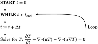
The simulation would evolve by an iterative
sequence which increases time  by an increment
 ,
then solves the equation, as shown below.
,
then solves the equation, as shown below.
Setting tolerances
The  equation is solved using an iterative
method such as Gauss-Seidel. Tolerance parameters determine when
the method stops iterating within the current solution step.
equation is solved using an iterative
method such as Gauss-Seidel. Tolerance parameters determine when
the method stops iterating within the current solution step.
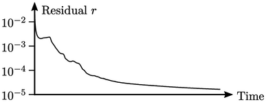
To capture the transient solution for
 accurately, the equation would need to converge to a suitable
absolute tolerance
accurately, the equation would need to converge to a suitable
absolute tolerance  at every time step. The question is: what
 is
suitable to give an accurate solution? — without setting it to a
very small value, e.g.
is
suitable to give an accurate solution? — without setting it to a
very small value, e.g.
 ,
which would would be highly inefficient, due to an excessive number
of solver iterations.
,
which would would be highly inefficient, due to an excessive number
of solver iterations.
Solution accuracy should be determined by some measure, or metric, e.g. temperature rise, pressure drop, drag coefficient, etc., relevant to the objective of the simulation.
The metric should be initially calculated using a
value of  , e.g.
  . It can then be
calculated again at a lower
. It can then be
calculated again at a lower  , typically decreasing
by one order of magnitude, i.e.
, typically decreasing
by one order of magnitude, i.e.  .
.
The metrics are then compared. If the difference
is within the required level of accuracy, then  is optimal. Otherwise,
 would need to be decreased further and the process repeated.
Residual calculation at intervals
The residual calculation of Eq. (5.11 ) incurs a significant computational cost since it involves multiplications of matrices. That cost can be reduced by setting an interval on the number of sweeps between residual calculations.
The downside is that convergence checks can only happen when the residual is calculated. If the residual is calculated at intervals of every second sweep, a solution that would otherwise converge at an odd number of sweeps is prolonged by a extra sweep.
Residuals are high when a simulation starts so a relatively high number of sweeps, e.g. 10, may be needed for convergence. The saving of calculating residuals at an interval may then offset the additional cost of unnecessary additional sweeps, giving a lower net cost per time step. However, as the residuals decrease and fewer sweeps are needed, attempts to reduce cost by intermittent residual calculation can be ineffective or counter-productive.
