
5.17 Multi-grid method
The methods for solving matrix equations described so far are Gauss-Seidel and CG. They are iterative, and require few iterations to calculate changes in the field, when the change at any given point is influenced only by points in the close vicinity.
This makes them efficient for solving equations
whose range of influence is limited, e.g. by the flow speed through advection
 in
a transport equation.
in
a transport equation.
The pressure equation contains neither a local
rate of change  nor advection term (assuming
  ). A disturbance at any
point influences the solution everywhere in the domain
instantaneously, as discussed in Sec. 4.3
.
). A disturbance at any
point influences the solution everywhere in the domain
instantaneously, as discussed in Sec. 4.3
.
To transfer changes across a domain, Gauss-Seidel might require as many sweeps as the number of cells across a domain, which would be impractical. Some method is therefore needed that transfers change across the domain more efficiently.
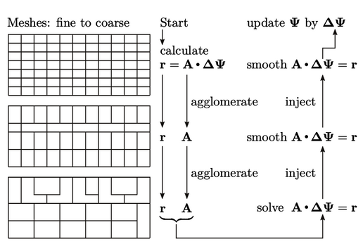
The multi-grid method6 uses a coarse mesh to overcome the problem of slow transfer of change across the domain, reducing the error at “low-frequency”. It transfers that solution through a succession of finer meshes to be accurate at higher frequencies.
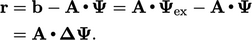
The multi-grid method works by first calculating
the matrix  and residual vector
  on the original
(finest) mesh. Coarser meshes are then successively formed until the
mesh reaches its coarsest level, containing as few as 10 cells.
on the original
(finest) mesh. Coarser meshes are then successively formed until the
mesh reaches its coarsest level, containing as few as 10 cells.
The matrix  and
and  are formed at each
level of coarsening. Different methods exist to calculate
are formed at each
level of coarsening. Different methods exist to calculate
 and
and  , including a simple agglomeration discussed in
Sec. 5.18
.
, including a simple agglomeration discussed in
Sec. 5.18
.
 , required to make
 exact, related to the residual
  by
by
 |
(5.36) |
 is solved precisely for
  , which can be
performed efficiently using a direct solver since the matrix is
small.
, which can be
performed efficiently using a direct solver since the matrix is
small.
 is then injected into the finer level, providing
the initial
is then injected into the finer level, providing
the initial  for a few sweeps of the Gauss-Seidel method at that
level. Smoothing and injection are repeated up to the finest level,
when the final
for a few sweeps of the Gauss-Seidel method at that
level. Smoothing and injection are repeated up to the finest level,
when the final  is applied to
  to yield the solution.
It is generally more efficient to do more Gauss-Seidel sweeps at the coarser levels, when the cost if low due to a smaller matrix size. For example, 4 sweeps may be applied at the coarser levels, while 2 sweeps are applied at the finest.
