[version 14][version 13][version 12][version 11][version 10][version 9][version 8][version 7][version 6]
2.2 Stress analysis of a plate with a hole
This tutorial describes how to pre-process, run
and post-process a case involving linear-elastic, steady-state
stress analysis on a square plate with a circular hole at its
centre. The plate dimensions are: side length 4  and radius
 0.5 . It is loaded with a uniform traction of
 10
10 
 over its left and right faces as shown in
Figure 2.16
. Two symmetry planes can
be identified for this geometry and therefore the solution domain
need only cover a quarter of the geometry, shown by the shaded area
in Figure 2.16
.
over its left and right faces as shown in
Figure 2.16
. Two symmetry planes can
be identified for this geometry and therefore the solution domain
need only cover a quarter of the geometry, shown by the shaded area
in Figure 2.16
.
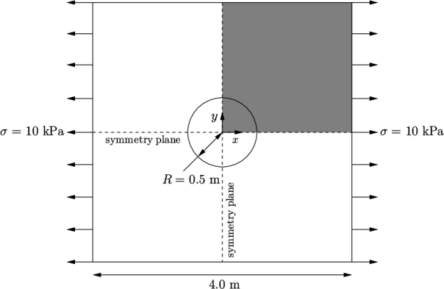
The problem can be approximated as 2-dimensional since the load is applied in the plane of the plate. In a Cartesian coordinate system there are two possible assumptions to take in regard to the behaviour of the structure in the third dimension: (1) the plane stress condition, in which the stress components acting out of the 2D plane are assumed to be negligible; (2) the plane strain condition, in which the strain components out of the 2D plane are assumed negligible. The plane stress condition is appropriate for solids whose third dimension is thin as in this case; the plane strain condition is applicable for solids where the third dimension is thick.
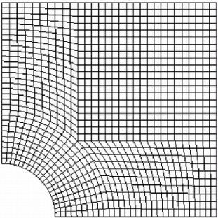
An analytical solution exists for loading of an infinitely large, thin plate with a circular hole. The solution for the stress normal to the vertical plane of symmetry is
 |
(2.14) |
2.2.1 Mesh generation
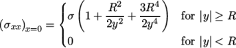
The domain consists of four blocks, some of
which have arc-shaped edges. The block structure for the part of
the mesh in the  plane is shown in Figure 2.17. As
already mentioned in section 2.1.1.1
, all geometries are
generated in 3 dimensions in OpenFOAM even if the case is to be as
a 2 dimensional problem. Therefore a dimension of the block in the
plane is shown in Figure 2.17. As
already mentioned in section 2.1.1.1
, all geometries are
generated in 3 dimensions in OpenFOAM even if the case is to be as
a 2 dimensional problem. Therefore a dimension of the block in the
 direction has to be chosen; here, 0.5
  is selected. It
does not affect the solution since the traction boundary condition
is specified as a stress rather than a force, thereby making the
solution independent of the cross-sectional area.
is selected. It
does not affect the solution since the traction boundary condition
is specified as a stress rather than a force, thereby making the
solution independent of the cross-sectional area.
The user should change to the run directory and copy the plateHole case into it from the $FOAM_TUTORIALS/stressAnalysis/solidDisplacementFoam directory. The user should then go into the plateHole directory and open the blockMeshDict file in an editor, as listed below
17
18vertices
19(
20 (0.5 0 0)
21 (1 0 0)
22 (2 0 0)
23 (2 0.707107 0)
24 (0.707107 0.707107 0)
25 (0.353553 0.353553 0)
26 (2 2 0)
27 (0.707107 2 0)
28 (0 2 0)
29 (0 1 0)
30 (0 0.5 0)
31 (0.5 0 0.5)
32 (1 0 0.5)
33 (2 0 0.5)
34 (2 0.707107 0.5)
35 (0.707107 0.707107 0.5)
36 (0.353553 0.353553 0.5)
37 (2 2 0.5)
38 (0.707107 2 0.5)
39 (0 2 0.5)
40 (0 1 0.5)
41 (0 0.5 0.5)
42);
43
44blocks
45(
46 hex (5 4 9 10 16 15 20 21) (10 10 1) simpleGrading (1 1 1)
47 hex (0 1 4 5 11 12 15 16) (10 10 1) simpleGrading (1 1 1)
48 hex (1 2 3 4 12 13 14 15) (20 10 1) simpleGrading (1 1 1)
49 hex (4 3 6 7 15 14 17 18) (20 20 1) simpleGrading (1 1 1)
50 hex (9 4 7 8 20 15 18 19) (10 20 1) simpleGrading (1 1 1)
51);
52
53edges
54(
55 arc 0 5 (0.469846 0.17101 0)
56 arc 5 10 (0.17101 0.469846 0)
57 arc 1 4 (0.939693 0.34202 0)
58 arc 4 9 (0.34202 0.939693 0)
59 arc 11 16 (0.469846 0.17101 0.5)
60 arc 16 21 (0.17101 0.469846 0.5)
61 arc 12 15 (0.939693 0.34202 0.5)
62 arc 15 20 (0.34202 0.939693 0.5)
63);
64
65boundary
66(
67 left
68 {
69 type symmetryPlane;
70 faces
71 (
72 (8 9 20 19)
73 (9 10 21 20)
74 );
75 }
76 right
77 {
78 type patch;
79 faces
80 (
81 (2 3 14 13)
82 (3 6 17 14)
83 );
84 }
85 down
86 {
87 type symmetryPlane;
88 faces
89 (
90 (0 1 12 11)
91 (1 2 13 12)
92 );
93 }
94 up
95 {
96 type patch;
97 faces
98 (
99 (7 8 19 18)
100 (6 7 18 17)
101 );
102 }
103 hole
104 {
105 type patch;
106 faces
107 (
108 (10 5 16 21)
109 (5 0 11 16)
110 );
111 }
112 frontAndBack
113 {
114 type empty;
115 faces
116 (
117 (10 9 4 5)
118 (5 4 1 0)
119 (1 4 3 2)
120 (4 7 6 3)
121 (4 9 8 7)
122 (21 16 15 20)
123 (16 11 12 15)
124 (12 13 14 15)
125 (15 14 17 18)
126 (15 18 19 20)
127 );
128 }
129);
130
131mergePatchPairs
132(
133);
134
135// ************************************************************************* //
Until now, we have only specified straight edges in the geometries of previous tutorials but here we need to specify curved edges. These are specified under the edges keyword entry which is a list of non-straight edges. The syntax of each list entry begins with the type of curve, including arc, simpleSpline, polyLine etc., described further in section 5.3.1 . In this example, all the edges are circular and so can be specified by the arc keyword entry. The following entries are the labels of the start and end vertices of the arc and a point vector through which the circular arc passes.
The blocks in this blockMeshDict do not all have the same orientation. As can be
seen in Figure 2.17
the  direction of block 0 is
equivalent to the
direction of block 0 is
equivalent to the  direction for block 4. This means care must be taken
when defining the number and distribution of cells in each block so
that the cells match up at the block faces.
direction for block 4. This means care must be taken
when defining the number and distribution of cells in each block so
that the cells match up at the block faces.
6 patches are defined: one for each side of the plate, one for the hole and one for the front and back planes. The left and down patches are both a symmetry plane. Since this is a geometric constraint, it is included in the definition of the mesh, rather than being purely a specification on the boundary condition of the fields. Therefore they are defined as such using a special symmetryPlane type as shown in the blockMeshDict.
The frontAndBack patch represents the plane which is ignored in a 2D case. Again this is a geometric constraint so is defined within the mesh, using the empty type as shown in the blockMeshDict. For further details of boundary types and geometric constraints, the user should refer to section 5.2 .
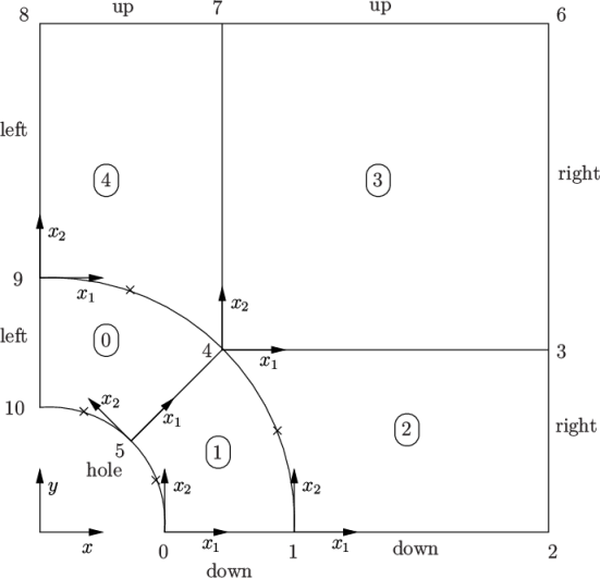
The remaining patches are of the regular patch type. The mesh should be generated using blockMesh and can be viewed in paraFoam as described in section 2.1.2 . It should appear as in Figure 2.18 .
2.2.1.1 Boundary and initial conditions
Once the mesh generation is complete, the initial field with boundary conditions must be set. For a stress analysis case without thermal stresses, only displacement D needs to be set. The 0/D is as follows:
17
18internalField uniform (0 0 0);
19
20boundaryField
21{
22 left
23 {
24 type symmetryPlane;
25 }
26 right
27 {
28 type tractionDisplacement;
29 traction uniform (10000 0 0);
30 pressure uniform 0;
31 value uniform (0 0 0);
32 }
33 down
34 {
35 type symmetryPlane;
36 }
37 up
38 {
39 type tractionDisplacement;
40 traction uniform (0 0 0);
41 pressure uniform 0;
42 value uniform (0 0 0);
43 }
44 hole
45 {
46 type tractionDisplacement;
47 traction uniform (0 0 0);
48 pressure uniform 0;
49 value uniform (0 0 0);
50 }
51 frontAndBack
52 {
53 type empty;
54 }
55}
56
57// ************************************************************************* //
Firstly, it can be seen that the displacement
initial conditions are set to 
 . The left and down patches must be both of symmetryPlane type since they are specified
as such in the mesh description in the constant/polyMesh/boundary file. Similarly
the frontAndBack patch is
declared empty.
. The left and down patches must be both of symmetryPlane type since they are specified
as such in the mesh description in the constant/polyMesh/boundary file. Similarly
the frontAndBack patch is
declared empty.
The other patches are traction boundary
conditions, set by a specialist traction boundary type. The traction
boundary conditions are specified by a linear combination of: (1) a
boundary traction vector under keyword traction; (2) a pressure that produces a traction normal to
the boundary surface that is defined as negative when pointing out
of the surface, under keyword pressure. The up and
hole patches are zero traction
so the boundary traction and pressure are set to zero. For the
right patch the traction should
be 
 and the pressure should be 0 .
2.2.1.2 Mechanical properties
The physical properties for the case are set in the mechanicalProperties dictionary in the constant directory. For this problem, we need to specify the mechanical properties of steel given in Table 2.1 . In the mechanical properties dictionary, the user must also set planeStress to yes.
| Property | Units | Keyword | Value |
|
|
|
|
|
| Density |  |
rho | 7854 |
| Young’s modulus |  |
E |  |
| Poisson’s ratio | — | nu | 0.3 |
|
|
|
|
|
2.2.1.3 Thermal properties
The temperature field variable T is present in the solidDisplacementFoam solver since the user may opt to solve a thermal equation that is coupled with the momentum equation through the thermal stresses that are generated. The user specifies at run time whether OpenFOAM should solve the thermal equation by the thermalStress switch in the thermophysicalProperties dictionary. This dictionary also sets the thermal properties for the case, e.g. for steel as listed in Table 2.2 .
| Property | Units | Keyword | Value |
|
|
|
|
|
| Specific heat capacity |    |
C | 434 |
| Thermal conductivity |    |
k | 60.5 |
| Thermal expansion coeff. | |
alpha |  |
|
|
|
|
|
In this case we do not want to solve for the thermal equation. Therefore we must set the thermalStress keyword entry to no in the thermophysicalProperties dictionary.
2.2.1.4 Control
As before, the information relating to the
control of the solution procedure are read in from the controlDict dictionary. For this case, the startTime is 0  . The time step is not
important since this is a steady state case; in this situation it
is best to set the time step deltaT to 1 so it simply acts as an
iteration counter for the steady-state case. The endTime, set to 100, then acts as a limit
on the number of iterations. The writeInterval can be set to
. The time step is not
important since this is a steady state case; in this situation it
is best to set the time step deltaT to 1 so it simply acts as an
iteration counter for the steady-state case. The endTime, set to 100, then acts as a limit
on the number of iterations. The writeInterval can be set to  .
.
The controlDict entries are as follows:
17application solidDisplacementFoam;
18
19startFrom startTime;
20
21startTime 0;
22
23stopAt endTime;
24
25endTime 100;
26
27deltaT 1;
28
29writeControl timeStep;
30
31writeInterval 20;
32
33purgeWrite 0;
34
35writeFormat ascii;
36
37writePrecision 6;
38
39writeCompression off;
40
41timeFormat general;
42
43timePrecision 6;
44
45graphFormat raw;
46
47runTimeModifiable true;
48
49
50// ************************************************************************* //
2.2.1.5 Discretisation schemes and linear-solver control
Let us turn our attention to the fvSchemes dictionary. Firstly, the problem we are analysing is steady-state so the user should select SteadyState for the time derivatives in timeScheme. This essentially switches off the time derivative terms. Not all solvers, especially in fluid dynamics, work for both steady-state and transient problems but solidDisplacementFoam does work, since the base algorithm is the same for both types of simulation.
The momentum equation in linear-elastic stress analysis includes several explicit terms containing the gradient of displacement. The calculations benefit from accurate and smooth evaluation of the gradient. Normally, in the finite volume method the discretisation is based on Gauss’s theorem. The Gauss method is sufficiently accurate for most purposes but, in this case, the least squares method will be used. The user should therefore open the fvSchemes dictionary in the system directory and ensure the leastSquares method is selected for the grad(U) gradient discretisation scheme in the gradSchemes sub-dictionary:
17d2dt2Schemes
18{
19 default steadyState;
20}
21
22ddtSchemes
23{
24 default Euler;
25}
26
27gradSchemes
28{
29 default leastSquares;
30 grad(D) leastSquares;
31 grad(T) leastSquares;
32}
33
34divSchemes
35{
36 default none;
37 div(sigmaD) Gauss linear;
38}
39
40laplacianSchemes
41{
42 default none;
43 laplacian(DD,D) Gauss linear corrected;
44 laplacian(kappa,T) Gauss linear corrected;
45}
46
47interpolationSchemes
48{
49 default linear;
50}
51
52snGradSchemes
53{
54 default none;
55}
56
57// ************************************************************************* //
The fvSolution dictionary in the system directory controls the linear
equation solvers and algorithms used in the solution. The user
should first look at the solvers sub-dictionary and notice that the
choice of solver for D is GAMG. The solver tolerance should be set to  for this problem. The
solver relative tolerance, denoted by relTol, sets the required reduction in the residuals
within each iteration. It is uneconomical to set a tight (low)
relative tolerance within each iteration since a lot of terms in
each equation are explicit and are updated as part of the
segregated iterative procedure. Therefore a reasonable value for
the relative tolerance is
for this problem. The
solver relative tolerance, denoted by relTol, sets the required reduction in the residuals
within each iteration. It is uneconomical to set a tight (low)
relative tolerance within each iteration since a lot of terms in
each equation are explicit and are updated as part of the
segregated iterative procedure. Therefore a reasonable value for
the relative tolerance is  , or possibly even higher, say
  , or in some
cases even
, or in some
cases even  (as in this case).
17solvers
18{
19 "(D|T)"
20 {
21 solver GAMG;
22 tolerance 1e-06;
23 relTol 0.9;
24 smoother GaussSeidel;
25 nCellsInCoarsestLevel 20;
26 }
27}
28
29stressAnalysis
30{
31 compactNormalStress yes;
32 nCorrectors 1;
33 D 1e-06;
34}
35
36
37// ************************************************************************* //
The fvSolution dictionary contains a sub-dictionary, stressAnalysis that contains some control parameters specific to the application solver. Firstly there is nCorrectors which specifies the number of outer loops around the complete system of equations, including traction boundary conditions within each time step. Since this problem is steady-state, we are performing a set of iterations towards a converged solution with the ’time step’ acting as an iteration counter. We can therefore set nCorrectors to 1.
The D keyword
specifies a convergence tolerance for the outer iteration loop,
i.e. sets a level of initial
residual below which solving will cease. It should be set to the
desired solver tolerance specified earlier,  for this problem.
2.2.2 Running the code
The user should run the code here in the background from the command line as specified below, so he/she can look at convergence information in the log file afterwards.
solidDisplacementFoam > log &
the run has converged
and can be stopped by killing the batch job.
2.2.3 Post-processing
Post processing can be performed as in
section 2.1.4
. The solidDisplacementFoam solver outputs the
stress field  as a symmetric tensor field sigma. This is consistent with the way
variables are usually represented in OpenFOAM solvers by the
mathematical symbol by which they are represented; in the case of
Greek symbols, the variable is named phonetically.
as a symmetric tensor field sigma. This is consistent with the way
variables are usually represented in OpenFOAM solvers by the
mathematical symbol by which they are represented; in the case of
Greek symbols, the variable is named phonetically.
For post-processing individual scalar field
components,  ,
,  etc., can be
generated by running the postProcess utility as before in
section 2.1.5.7
, this time on
sigma:
etc., can be
generated by running the postProcess utility as before in
section 2.1.5.7
, this time on
sigma:
postProcess -func "components(sigma)"
 stresses can be viewed in paraFoam as shown in
Figure 2.19
.
stresses can be viewed in paraFoam as shown in
Figure 2.19
.
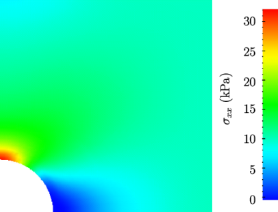
 stress field in the plate with
hole.
stress field in the plate with
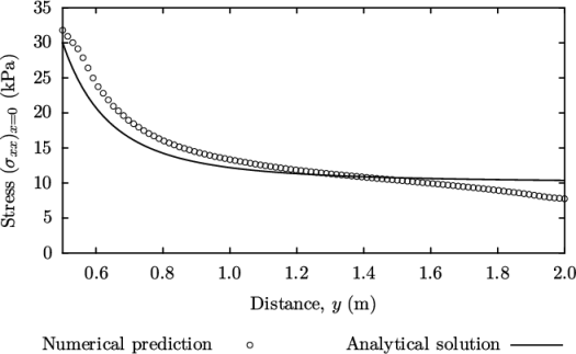
hole.We would like to compare the analytical solution
of Equation 2.14
to our solution. We
therefore must output a set of data of  along the left edge
symmetry plane of our domain. The user may generate the required
graph data using the postProcess utility with the graphUniform function. Unlike earlier
examples of postProcess where
no configuration is required, this example includes a graphUniform file pre-configured in the
system directory. The sample
line is set between
along the left edge
symmetry plane of our domain. The user may generate the required
graph data using the postProcess utility with the graphUniform function. Unlike earlier
examples of postProcess where
no configuration is required, this example includes a graphUniform file pre-configured in the
system directory. The sample
line is set between  and
and  , and the fields are specified in the
fields list:
, and the fields are specified in the
fields list:
10 end points. A specified number of graph points are used, distributed
11 uniformly along the line.
12
13\*---------------------------------------------------------------------------*/
14
15start (0 0.5 0.25);
16end (0 2 0.25);
17nPoints 100;
18
19fields (sigmaxx);
20
21axis y;
22
23#includeEtc "caseDicts/postProcessing/graphs/graphUniform.cfg"
24
25// ************************************************************************* //
The user should execute postProcessing with the graphUniform function:
postProcess -func graphUniform
 s is found within the file graphUniform/100/line_sigmaxx.xy. If the user has GnuPlot installed they launch it (by typing
gnuplot) and then plot both the
numerical data and analytical solution as follows:
s is found within the file graphUniform/100/line_sigmaxx.xy. If the user has GnuPlot installed they launch it (by typing
gnuplot) and then plot both the
numerical data and analytical solution as follows:
plot [0.5:2] [0:] "postProcessing/graphUniform/100/line_sigmaxx.xy",
1e4*(1+(0.125/(x**2))+(0.09375/(x**4)))

2.2.4 Exercises
The user may wish to experiment with solidDisplacementFoam by trying the following exercises:
2.2.4.1 Increasing mesh resolution
Increase the mesh resolution in each of the
 and
and
 directions. Use mapFields to map the final coarse mesh
results from section 2.2.3
to the initial conditions
for the fine mesh.
directions. Use mapFields to map the final coarse mesh
results from section 2.2.3
to the initial conditions
for the fine mesh.
2.2.4.2 Introducing mesh grading
Grade the mesh so that the cells near the hole are finer than those away from the hole. Design the mesh so that the ratio of sizes between adjacent cells is no more than 1.1 and so that the ratio of cell sizes between blocks is similar to the ratios within blocks. Mesh grading is described in section 2.1.6 . Again use mapFields to map the final coarse mesh results from section 2.2.3 to the initial conditions for the graded mesh. Compare the results with those from the analytical solution and previous calculations. Can this solution be improved upon using the same number of cells with a different solution?
2.2.4.3 Changing the plate size
The analytical solution is for an infinitely large plate with a finite sized hole in it. Therefore this solution is not completely accurate for a finite sized plate. To estimate the error, increase the plate size while maintaining the hole size at the same value.