OpenFOAM v9 User Guide

[version 12][version 11][version 10][version 9][version 8][version 7][version 6]

[chapter contents][previous topic][next topic][index]

5.2 Boundaries

In this section we discuss the way in which boundaries are treated in OpenFOAM. The subject of boundaries is quite complex because their role in modelling is not simply that of a geometric entity but an integral part of the solution and numerics through boundary conditions or inter-boundary ‘connections’. A discussion of boundaries sits uncomfortably between a discussion on meshes, ﬁelds, discretisation, computational processing etc.

We ﬁrst need to consider that, for the purpose of applying boundary conditions, a boundary is generally broken up into a set of patches. One patch may include one or more enclosed areas of the boundary surface which do not necessarily need to be physically connected. A type is assigned to every patch as part of the mesh description, as part of the boundary ﬁle described in section 5.1.2 . It describes the type of patch in terms of geometry or a data ‘communication link’. An example boundary ﬁle is shown below for a rhoPimpleFoam case. A type entry is clearly included for every patch (inlet, outlet, etc.), with types assigned that include patch, symmetryPlane and empty.

16// * * * * * * * * * * * * * * * * * * * * * * * * * * * * * * * * * * * * * //
17
186
19(
20    inlet
21    {
22        type            patch;
23        nFaces          50;
24        startFace       10325;
25    }
26    outlet
27    {
28        type            patch;
29        nFaces          40;
30        startFace       10375;
31    }
32    bottom
33    {
34        type            symmetryPlane;
35        inGroups        1(symmetryPlane);
36        nFaces          25;
37        startFace       10415;
38    }
39    top
40    {
41        type            symmetryPlane;
42        inGroups        1(symmetryPlane);
43        nFaces          125;
44        startFace       10440;
45    }
46    obstacle
47    {
48        type            patch;
49        nFaces          110;
50        startFace       10565;
51    }
52    defaultFaces
53    {
54        type            empty;
55        inGroups        1(empty);
56        nFaces          10500;
57        startFace       10675;
58    }
59)
60
61// ************************************************************************* //

The user can scan the tutorials for mesh generation conﬁguration ﬁles, e.g. blockMeshDict for blockMesh (see section 5.3 ) and snappyHexMeshDict for snappyHexMesh (see section 5.4 , for examples of diﬀerent types being used. The following example provides documentation and lists cases that use the symmetryPlane condition.

foamInfo -a symmetryPlane

The next example searches for snappyHexMeshDict ﬁles that specify the wall condition.

find $FOAM_TUTORIALS -name snappyHexMeshDict | \
xargs grep -El "type[\t ]*wall"

$wedge patch 2 <5 ∘ Axis of symmetry wedge patch 1 wedge aligned along coordinate plane \relax \special {t4ht=$

Figure 5.3: Axi-symmetric geometry using the wedge patch type.

5.2.1 Geometric (constraint) patch types

The main geometric types available in OpenFOAM are summarised below. This is not a complete list; for all types see $FOAM_SRC/ﬁniteVolume/ﬁelds/fvPatchFields/constraint.

patch : generic type containing no geometric or topological information about the mesh, e.g. used for an inlet or an outlet.
wall : for patch that coincides with a solid wall, required for some physical modelling, e.g. wall functions in turbulence modelling.
symmetryPlane : for a planar patch which is a symmetry plane.
symmetry : for any (non-planar) patch which uses the symmetry plane (slip) condition.
empty : for solutions in in 2 (or 1) dimensions (2D/1D), the type used on each patch whose plane is normal to the 3rd (and 2nd) dimension for which no solution is required.
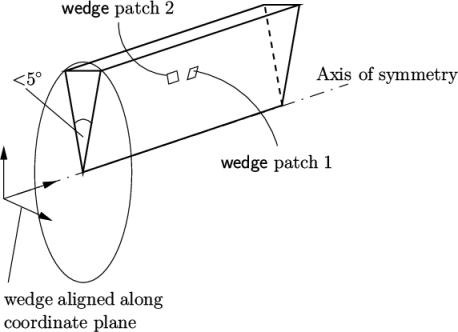
wedge : for 2 dimensional axi-symmetric cases, e.g. a cylinder, the geometry is speciﬁed as a wedge of small angle (e.g. $\text{[math]}$ ) and 1 cell thick, running along the centre line, straddling one of the coordinate planes, as shown in Figure 5.3 ; the axi-symmetric wedge planes must be speciﬁed as separate patches of wedge type.
cyclic : enables two patches to be treated as if they are physically connected; used for repeated geometries; one cyclic patch is linked to another through a neighbourPatch keyword in the boundary ﬁle; each pair of connecting faces must have similar area to within a tolerance given by the matchTolerance keyword in the boundary ﬁle.
cyclicAMI : like cyclic, but for 2 patches whose faces are non matching; used for sliding interface in rotating geometry cases.
processor : the type that describes inter-processor boundaries for meshes decomposed for parallel running.

5.2.2 Basic boundary conditions

Boundary conditions are speciﬁed in ﬁeld ﬁles, e.g. p, U, in time directories as described in section 4.2.8 . An example pressure ﬁeld ﬁle, p, is shown below for the rhoPimpleFoam case corresponding to the boundary ﬁle presented in section 5.2.1 .

16dimensions      [1 -1 -2 0 0 0 0];
17
18internalField   uniform 1;
19
20boundaryField
21{
22    inlet
23    {
24        type            fixedValue;
25        value           uniform 1;
26    }
27
28    outlet
29    {
30        type            waveTransmissive;
31        field           p;
32        psi             thermo:psi;
33        gamma           1.4;
34        fieldInf        1;
35        lInf            3;
36        value           uniform 1;
37    }
38
39    bottom
40    {
41        type            symmetryPlane;
42    }
43
44    top
45    {
46        type            symmetryPlane;
47    }
48
49    obstacle
50    {
51        type            zeroGradient;
52    }
53
54    defaultFaces
55    {
56        type            empty;
57    }
58}
59
60// ************************************************************************* //

Every patch includes a type entry that speciﬁes the type of boundary condition. They range from a basic fixedValue condition applied to the inlet, to a complex waveTransmissive condition applied to the outlet. The patches with non-generic types, e.g. symmetryPlane, deﬁned in boundary, use consistent boundary condition types in the p ﬁle.

The main basic boundary condition types available in OpenFOAM are summarised below using a patch ﬁeld named $\text{[math]}$ . This is not a complete list; for all types see $FOAM_SRC/ﬁniteVolume/ﬁelds/fvPatchFields/basic.

ﬁxedValue : value of $\text{[math]}$ is speciﬁed by value .
ﬁxedGradient : normal gradient of $\text{[math]}$ ( $\text{[math]}$ ) is speciﬁed by gradient.
zeroGradient : normal gradient of $\text{[math]}$ is zero.
calculated : patch ﬁeld $\text{[math]}$ calculated from other patch ﬁelds.
mixed : mixed ﬁxedValue/ ﬁxedGradient condition depending on valueFraction $\text{[math]}$ where

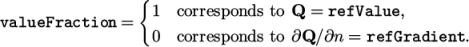
${ 1 corresponds to Q = refValue, valueFraction = 0 corresponds to ∂Q ∕∂n = refGradient. \relax \special {t4ht=$ (5.1)
directionMixed : mixed condition with tensorial valueFraction , to allow diﬀerent conditions in normal and tangential directions of a vector patch ﬁeld, e.g. ﬁxedValue in the tangential direction, zeroGradient in the normal direction.

5.2.3 Derived types

There are numerous more complex boundary conditions derived from the basic conditions. For example, many complex conditions are derived from ﬁxedValue, where the value is calculated by a function of other patch ﬁelds, time, geometric information, etc. Some other conditions derived from mixed/directionMixed switch between ﬁxedValue and ﬁxedGradient (usually zeroGradient).

There are a number of ways the user can list the available boundary conditions in OpenFOAM, with the -listScalarBCs and -listVectorBCs utility being the quickest. The boundary conditions for scalar ﬁelds and vector ﬁelds, respectively, can be listed for a given solver, e.g. simpleFoam, as follows.

simpleFoam -listScalarBCs -listVectorBCs

These produce long lists which the user can scan through. If the user wants more information of a particular condition, they can run the foamInfo script which provides a description of the boundary condition and lists example cases where it is used. For example, for the totalPressure boundary condition, run the following.

foamInfo totalPressure

In the following sections we will highlight some particular important, commonly used boundary conditions.

5.2.3.1 The inlet/outlet condition

The inletOutlet condition is one derived from mixed, which switches between zeroGradient when the ﬂuid ﬂows out of the domain at a patch face, and ﬁxedValue, when the ﬂuid is ﬂowing into the domain. For inﬂow, the inlet value is speciﬁed by an inletValue entry. A good example of its use can be seen in the damBreak tutorial, where it is applied to the phase fraction on the upper atmosphere boundary. Where there is outﬂow, the condition is well posed, where there is inﬂow, the phase fraction is ﬁxed with a value of 0, corresponding to 100% air.

16dimensions      [0 0 0 0 0 0 0];
17
18internalField   uniform 0;
19
20boundaryField
21{
22    leftWall
23    {
24        type            zeroGradient;
25    }
26
27    rightWall
28    {
29        type            zeroGradient;
30    }
31
32    lowerWall
33    {
34        type            zeroGradient;
35    }
36
37    atmosphere
38    {
39        type            inletOutlet;
40        inletValue      uniform 0;
41        value           uniform 0;
42    }
43
44    defaultFaces
45    {
46        type            empty;
47    }
48}
49
50// ************************************************************************* //

5.2.3.2 Entrainment boundary conditions

The combination of the totalPressure condition on pressure and pressureInletOutletVelocity on velocity is extremely common for patches where some inﬂow occurs and the inlet ﬂow velocity is not known. That includes the atmosphere boundary in the damBreak tutorial, inlet conditions where only pressure is known, outlets where ﬂow reversal may occur, and where ﬂow in entrained, e.g. on boundaries surrounding a jet through a nozzle.

The totalPressure condition speciﬁes

{ p for outﬂow p = 0 1 2 p0 − 2|U | for inﬂow (incompressible, subsonic) \relax \special {t4ht=

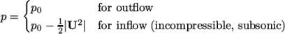(5.2)

where the user speciﬁes $\text{[math]}$ through the p0 keyword. The pressureInletOutletVelocity condition speciﬁes zeroGradient at all times, except on the tangential component which is set to ﬁxedValue for inﬂow, with the tangentialVelocity defaulting to 0.

The idea behind this combination is that the condition is a standard combination in the case of outﬂow, but for inﬂow the normal velocity is allowed to ﬁnd its own value. Under these circumstances, a rapid rise in velocity presents a risk of instability, but the rise is moderated by the reduction of inlet pressure, and hence driving pressure gradient, as the inﬂow velocity increases.

The speciﬁcation of these boundary conditions in the U and p_rgh ﬁles, in the damBreak case, are shown below.

16
17dimensions      [0 1 -1 0 0 0 0];
18
19internalField   uniform (0 0 0);
20
21boundaryField
22{
23    leftWall
24    {
25        type            noSlip;
26    }
27    rightWall
28    {
29        type            noSlip;
30    }
31    lowerWall
32    {
33        type            noSlip;
34    }
35    atmosphere
36    {
37        type            pressureInletOutletVelocity;
38        value           uniform (0 0 0);
39    }
40    defaultFaces
41    {
42        type            empty;
43    }
44}
45
46
47// ************************************************************************* //

16dimensions      [1 -1 -2 0 0 0 0];
17
18internalField   uniform 0;
19
20boundaryField
21{
22    leftWall
23    {
24        type            fixedFluxPressure;
25        value           uniform 0;
26    }
27
28    rightWall
29    {
30        type            fixedFluxPressure;
31        value           uniform 0;
32    }
33
34    lowerWall
35    {
36        type            fixedFluxPressure;
37        value           uniform 0;
38    }
39
40    atmosphere
41    {
42        type            totalPressure;
43        p0              uniform 0;
44    }
45
46    defaultFaces
47    {
48        type            empty;
49    }
50}
51
52// ************************************************************************* //

5.2.3.3 Fixed ﬂux pressure

In the above example, it can be seen that all the wall boundaries use a boundary condition named ﬁxedFluxPressure. This boundary condition is used for pressure in situations where zeroGradient is generally used, but where body forces such as gravity and surface tension are present in the solution equations. The condition adjusts the gradient accordingly.

5.2.3.4 Time-varying boundary conditions

There are several boundary conditions for which some input parameters are speciﬁed by a function of time (using Function1 functionality) class. They can be searched by the following command.

find $FOAM_SRC/finiteVolume/fields/fvPatchFields -type f -name "*.H" |\
xargs grep -l Function1 | xargs dirname | sort

They include conditions such as uniformFixedValue , which is a ﬁxedValue condition which applies a single value which is a function of time through a uniformValue keyword entry.

The Function1 is speciﬁed by a keyword following the uniformValue entry, followed by parameters that relate to the particular function. The Function1 options are list below.

constant : constant value.
table : inline list of (time value) pairs; interpolates values linearly between times.
tableFile : as above, but with data supplied in a separate ﬁle.
square : square-wave function.
squarePulse : single square pulse.
sine : sine function.
one and zero : constant one and zero values.
polynomial : polynomial function using a list (coeff exponent) pairs.
coded : function speciﬁed by user coding.
scale : scales a given value function by a scalar scale function; both entries can be themselves Function1; scale function is often a ramp function (below), with value controlling the ramp value.
linearRamp , quadraticRamp , halfCosineRamp , quarterCosineRamp and quarterSineRamp : monotonic ramp functions which ramp from 0 to 1 over speciﬁed duration.
reverseRamp : reverses the values of a ramp function, e.g. from 1 to 0.

Examples or a time-varying inlet for a scalar are shown below.

inlet
{
    type         uniformFixedValue;
    uniformValue constant 2;
}

inlet
{
    type         uniformFixedValue;
    uniformValue table ((0 0) (10 2));
}

inlet
{
    type         uniformFixedValue;
    uniformValue polynomial ((1 0) (2 2)); // = 1*t^0 + 2*t^2
}

inlet
{
    type         uniformFixedValue;
    uniformValue
    {
        type             tableFile;
        format           csv;
        nHeaderLine      4;              // number of header lines
        refColumn        0;              // time column index
        componentColumns (1);            // data column index
        separator        ",";            // optional (defaults to ",")
        mergeSeparators  no;             // merge multiple separators
        file             "dataTable.csv";
   }
}

inlet
{
    type         uniformFixedValue;
    uniformValue
    {
        type             square;
        frequency        10;
        amplitude        1;
        scale            2;  // Scale factor for wave
        level            1;  // Offset
    }
}

inlet
{
    type         uniformFixedValue;
    uniformValue
    {
        type             sine;
        frequency        10;
        amplitude        1;
        scale            2;  // Scale factor for wave
        level            1;  // Offset
    }
}

input  // ramp from 0 -> 2, from t = 0 -> 0.4
{
    type         uniformFixedValue;
    uniformValue
    {
        type             scale;
        scale            linearRamp;
        start            0;
        duration         0.4;
        value            2;
    }
}

input  // ramp from 2 -> 0, from t = 0 -> 0.4
{
    type         uniformFixedValue;
    uniformValue
    {
        type             scale;
        scale            reverseRamp;
ramp             linearRamp;
        start            0;
        duration         0.4;
        value            2;
    }
}

inlet  // pulse with value 2, from t = 0 -> 0.4
{
    type         uniformFixedValue;
    uniformValue
    {
        type             scale;
scale            squarePulse
        start            0;
        duration         0.4;
        value            2;
    }
}

inlet
{
    type            uniformFixedValue;
    uniformValue    coded;
    name            pulse;
    codeInclude
    #{
        #include "mathematicalConstants.H"
    #};

    code
    #{
        return scalar
        (
            0.5*(1 - cos(constant::mathematical::twoPi*min(x/0.3, 1)))
        );
    #};
}

OpenFOAM v9 User Guide - 5.2 Boundaries