OpenFOAM v10 User Guide

[version 11][version 10][version 9][version 8][version 7][version 6]

[chapter contents][previous topic][index]

7.3 Transport/rheology models

In OpenFOAM, simulations that include ﬂow without energy/heat require modelling of the ﬂuid stress. Many simulations assume a Newtonian ﬂuid in which a viscosity $\text{[math]}$ is speciﬁed in physicalProperties, e.g. by

viscosityModel constant;

nu 1.5e-05;

This viscosity is a single value which is constant in time and uniform over the solution domain. Non-Newtonian models can be speciﬁed in the momentumTransport ﬁle, including:

a family of generalisedNewtonian models for a non-uniform viscosity which is a function of strain rate $\text{[math]}$ , described in sections 7.3.1 , 7.3.2, 7.3.3 , 7.3.4 , 7.3.5 and 7.3.6 ;
a set of visco-elastic models, including Maxwell , Giesekus and PTT (Phan-Thien & Tanner), described in sections 7.3.7 , 7.3.8 and 7.3.9 , respectively;
the lambdaThixotropic model, described in section 7.3.10 .

7.3.1 Bird-Carreau model

The Bird-Carreau generalisedNewtonian model is

a(n−1)∕a ν = ν∞ + (ν0 − ν∞)[1 + (k ˙γ) ] \relax \special {t4ht=

(7.22)

where the coeﬃcient $\text{[math]}$ has a default value of 2. An example speciﬁcation of the model in momentumTransport is:

viscosityModel BirdCarreau;

nuInf   1e-05;
k       1;
n       0.5;

The constant, uniform viscosity at zero strain-rate, $\text{[math]}$ , is speciﬁed in the physicalProperties ﬁle.

7.3.2 Cross Power Law model

The Cross Power Law generalisedNewtonian model is:

ν − ν ν = ν∞ + --0----∞n- 1 + (m γ˙) \relax \special {t4ht=

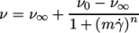(7.23)

An example speciﬁcation of the model in momentumTransport is:

viscosityModel CrossPowerLaw;

nuInf   1e-05;
m       1;
n       0.5;

The constant, uniform viscosity at zero strain-rate, $\text{[math]}$ , is speciﬁed in the physicalProperties ﬁle.

7.3.3 Power Law model

The Power Law generalisedNewtonian model provides a function for viscosity, limited by minimum and maximum values, $\text{[math]}$ and $\text{[math]}$ respectively. The function is:

ν = k˙γn− 1 νmin ≤ ν ≤ νmax \relax \special {t4ht=

(7.24)

An example speciﬁcation of the model in momentumTransport is:

viscosityModel powerLaw;

nuMax    1e-03;
nuMin    1e-05;
k        1e-05;
n        0.5;

7.3.4 Herschel-Bulkley model

The Herschel-Bulkley generalisedNewtonian model combines the eﬀects of Bingham plastic and power-law behavior in a ﬂuid. For low strain rates, the material is modelled as a very viscous ﬂuid with viscosity $\text{[math]}$ . Beyond a threshold in strain-rate corresponding to threshold stress $\text{[math]}$ , the viscosity is described by a power law. The model is:

( n− 1) ν = min ν0,τ0∕γ˙+ k˙γ \relax \special {t4ht=

(7.25)

An example speciﬁcation of the model in momentumTransport is:

viscosityModel HerschelBulkley;

tau0     0.01;
k        0.001;
n        0.5;

The constant, uniform viscosity at zero strain-rate, $\text{[math]}$ , is speciﬁed in the physicalProperties ﬁle.

7.3.5 Casson model

The Casson generalisedNewtonian model is a basic model used in blood rheology that speciﬁes minimum and maximum viscosities, $\text{[math]}$ and $\text{[math]}$ respectively. Beyond a threshold in strain-rate corresponding to threshold stress $\text{[math]}$ , the viscosity is described by a “square-root” relationship. The model is:

( ) ν = ∘ τ-∕˙γ-+ √m- 2 ν ≤ ν ≤ ν 0 min max \relax \special {t4ht=

(7.26)

An example speciﬁcation of model parameters for blood is:

viscosityModel Casson;

m        3.934986e-6;
tau0     2.9032e-6;
nuMax    13.3333e-6;
nuMin    3.9047e-6;

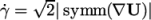
7.3.6 General strain-rate function

A strainRateFunction generalisedNewtonian model exists that allows a user to specify viscosity as a function of strain rate at run-time. It uses the same Function1 functionality to specify the function of strain-rate, used by time varying properties in boundary conditions described in section 5.2.3.4 . An example speciﬁcation of the model in momentumTransport is shown below using the polynomial function:

viscosityModel strainRateFunction;

function polynomial ((0 0.1) (1 1.3));

7.3.7 Maxwell model

The Maxwell laminar visco-elastic model solves an equation for the ﬂuid stress tensor $\text{[math]}$ :

∂-τ+ ∇ ∙(U τ) = 2 symm [τ∙∇U ]− 2νM-symm (∇U )− 1τ ∂t λ λ \relax \special {t4ht=

(7.27)

where $\text{[math]}$ (nuM) is the “Maxwell” viscosity and $\text{[math]}$ (lambda) is the relaxation time. An example speciﬁcation of model parameters is shown below:

simulationType laminar;

laminar
{
    model               Maxwell;

    MaxwellCoeffs
    {
        nuM             0.002;
        lambda          0.03;
    }
}

If an additional constant, uniform viscosity at zero strain-rate, $\text{[math]}$ , is speciﬁed in the physicalProperties ﬁle, the model becomes equivalent to an Oldroyd-B visco-elastic model. The Maxwell model includes a multi-mode option where $\text{[math]}$ is a sum of stresses, each with an associated relaxation time $\text{[math]}$ .

7.3.8 Giesekus model

The Giesekus laminar visco-elastic model is similar to the Maxwell model but includes an additional “mobility” term in the equation for $\text{[math]}$ :

∂ τ ν 1 α ---+ ∇ ∙(U τ) = 2 symm [τ∙∇U ]− 2-M- symm (∇U ) − -τ − -G-[τi∙τi] ∂t λ λ νM \relax \special {t4ht=

(7.28)

where $\text{[math]}$ (alphaG) is the mobility parameter. An example speciﬁcation of model parameters is shown below:

simulationType laminar;

laminar
{
    model               Giesekus;

    GiesekusCoeffs
    {
        nuM             0.002;
        lambda          0.03;
        alphaG          0.1;
    }
}

The Giesekus model includes a multi-mode option where $\text{[math]}$ is a sum of stresses, each with an associated relaxation time $\text{[math]}$ and mobility coeﬃcient $\text{[math]}$ .

7.3.9 Phan-Thien-Tanner (PTT) model

The Phan-Thien-Tanner (PTT) laminar visco-elastic model is also similar to the Maxwell model but includes an additional “extensibility” term in the equation for $\text{[math]}$ , suitable for polymeric liquids:

∂τ νM 1 ( 𝜀λ ) ---+ ∇ ∙(Uτ) = 2symm [τ∙∇U ]− 2---symm (∇U )− -exp − ---tr(τ) τ ∂t λ λ νM \relax \special {t4ht=

(7.29)

where $\text{[math]}$ (epsilon) is the extensibility parameter. An example speciﬁcation of model parameters is shown below:

simulationType laminar;

laminar
{
    model               PTT;

    PTTCoeffs
    {
        nuM             0.002;
        lambda          0.03;
        epsilon         0.25;
    }
}

The PTT model includes a multi-mode option where $\text{[math]}$ is a sum of stresses, each with an associated relaxation time $\text{[math]}$ and extensibility coeﬃcient $\text{[math]}$ .

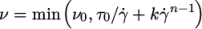
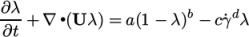
7.3.10 Lambda thixotropic model

The Lambda Thixotropic laminar model calculates the evolution of a structural parameter $\text{[math]}$ (lambda) according to:

∂λ-+ ∇ ∙(U λ) = a (1 − λ)b − cγ˙dλ ∂t \relax \special {t4ht=

(7.30)

with model coeﬃcients $\text{[math]}$ , $\text{[math]}$ , $\text{[math]}$ and $\text{[math]}$ . The viscosity $\text{[math]}$ is then calculated according to:

ν ν = ----∞--2 1 − K λ \relax \special {t4ht=

(7.31)

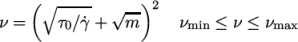
where the parameter $\text{[math]}$ . The viscosities $\text{[math]}$ and $\text{[math]}$ are limiting values corresponding to $\text{[math]}$ and $\text{[math]}$ .

An example speciﬁcation of the model in momentumTransport is:

simulationType laminar;

laminar
{
    model               lambdaThixotropic;

    lambdaThixotropicCoeffs
    {
        a       1;
        b       2;
        c       1e-3;
        d       3;
        nu0     0.1;
        nuInf   1e-4;
    }
}

OpenFOAM v10 User Guide - 7.3 Transport/rheology models