[version 13][version 12][version 11][version 10][version 9][version 8][version 7][version 6]
7.1 Thermophysical models
Thermophysical models are concerned with:
thermodynamics, e.g. relating
internal energy  to temperature
  ; transport,
e.g. the dependence of
properties such as
; transport,
e.g. the dependence of
properties such as  on temperature; and state, e.g. dependence of density
  on
on  and pressure
 .
Thermophysical models are specified in the physicalProperties dictionary.
.
Thermophysical models are specified in the physicalProperties dictionary.
A thermophysical model required an entry named thermoType which specifies the package of thermophysical modelling that is used in the simulation. OpenFOAM includes a large set of pre-compiled combinations of modelling, built within the code using C++ templates. It can also compile on-demand a combination which is not pre-compiled during a simulation.
Thermophysical modelling packages begin with the equation of state and then adding more layers of thermophysical modelling that derive properties from the previous layer(s). The keyword entries in thermoType reflects the multiple layers of modelling and the underlying framework in which they combined. Below is an example entry for thermoType:
thermoType
{
type hePsiThermo;
mixture pureMixture;
transport const;
thermo hConst;
equationOfState perfectGas;
specie specie;
energy sensibleEnthalpy;
}
The keyword entries specify the choice of thermophysical models, e.g. transport constant (constant viscosity, thermal diffusion), equationOfState perfectGas , etc. In addition there is a keyword entry named energy that allows the user to specify the form of energy to be used in the solution and thermodynamics. The following sections explains the entries and options in the thermoType package.
7.1.1 Thermophysical and mixture models
Each solver that uses thermophysical modelling constructs an object of a specific thermophysical model class. The model classes are listed below.
- fluidThermo
- Thermophysical model for a general fluid with fixed composition. The solvers using fluidThermo are rhoSimpleFoam, rhoPorousSimpleFoam rhoPimpleFoam, buoyantFoam, rhoParticleFoam and thermoFoam.
- psiThermo
- Thermophysical model for gases only, with fixed composition, used by rhoCentralFoam.
- fluidReactionThermo
- Thermophysical model for fluid of varying composition, including reactingFoam, chtMultiRegionFoam and chemFoam.
- psiuReactionThermo
- Thermophysical model for combustion solvers that model combustion based on laminar flame speed and regress variable, e.g.XiFoam, PDRFoam.
- multiphaseMixtureThermo
- Thermophysical models for multiple phases used by compressibleMultiphaseInterFoam.
- solidThermo
- Thermophysical models for solids used by chtMultiRegionFoam.
The type keyword (in the thermoType sub-dictionary) specifies the underlying thermophysical model used by the solver. The user can select from the following.
- hePsiThermo: available for solvers that construct fluidThermo, fluidReactionThermo and psiThermo.
- heRhoThermo: available for solvers that construct fluidThermo, fluidReactionThermo and multiphaseMixtureThermo.
- heheuPsiThermo: for solvers that construct psiuReactionThermo.
- heSolidThermo: for solvers that construct solidThermo.
The mixture specifies the mixture composition. The option typically used for thermophysical models without reactions is pureMixture, which represents a mixture with fixed composition. When pureMixture is specified, the thermophysical models coefficients are specified within a sub-dictionary called mixture.
For mixtures with variable composition, required by thermophysical models with reactions, the multicomponentMixture option is used. Species and reactions are listed in a chemistry file, specified by the foamChemistryFile keyword. The multicomponentMixture model then requires the thermophysical models coefficients to be specified for each specie within sub-dictionaries named after each specie, e.g. O2, N2.
For combustion based on laminar flame speed and regress variables, constituents are a set of mixtures, such as fuel, oxidant and burntProducts. The available mixture models for this combustion modelling are homogeneousMixture, inhomogeneousMixture and veryInhomogeneousMixture.
Other models for variable composition are egrMixture, singleComponentMixture.
7.1.2 Transport model
The transport modelling
concerns evaluating dynamic viscosity  , thermal conductivity
 and
thermal diffusivity
and
thermal diffusivity  (for internal energy and enthalpy equations).
The current transport models
are as follows:
(for internal energy and enthalpy equations).
The current transport models
are as follows:
- const
- assumes a constant
 and Prandtl number
 which is simply specified by a two keywords, mu and Pr, respectively.
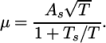
 - sutherland
- calculates as a function of
temperature
 from a Sutherland coefficient
  and Sutherland
temperature
and Sutherland
temperature  , specified by keywords As and Ts;
  is calculated according
to:
is calculated according
to:
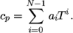
(7.1) - polynomial
- calculates and
 as a function of
temperature
as a function of
temperature  from a polynomial of any order
  , e.g.:

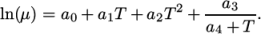
(7.2) - logPolynomial
- calculates
 and
and  as a function of
 from a polynomial of any order
  ; from which
 ,
,
 are
calculated by taking the exponential, e.g.:
are
calculated by taking the exponential, e.g.:
![N∑−1 ln(μ) = ai[ln (T )]i. i=0 \relax \special {t4ht=](img/index451x.png)
(7.3) - Andrade
- calculates
 and
and  as a polynomial
function of
as a polynomial
function of  , e.g. for
 :
:
(7.4) - tabulated
- uses uniform tabulated data for viscosity and thermal conductivity as a function of pressure and temperature.
- icoTabulated
- uses non-uniform tabulated data for viscosity and thermal conductivity as a function of temperature.
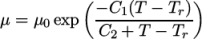
- WLF
- (Williams-Landel-Ferry) calculates
as
a function of temperature from coefficients
 and
and  and reference
temperature
and reference
temperature  specified by keywords C1, C2 and Tr;
  is calculated according to:
(7.5)
7.1.3 Thermodynamic models
The thermodynamic
models are concerned with evaluating the specific heat  from which
other properties are derived. The current thermo models are as follows:
from which
other properties are derived. The current thermo models are as follows:
- eConst
- assumes a constant
 and a heat of fusion
 which is simply specified by a two values
  , given by keywords
Cv and Hf.
, given by keywords
Cv and Hf. - eIcoTabulated
- calculates
 by interpolating
non-uniform tabulated data of
by interpolating
non-uniform tabulated data of  value pairs,
e.g.:
value pairs,
e.g.:
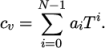
( (200 1005) (400 1020) ); - ePolynomial
- calculates
 as a function of
temperature by a polynomial of any order
as a function of
temperature by a polynomial of any order  :
:
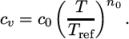
(7.6) - ePower
- calculates
 as a power of
temperature according to:
as a power of
temperature according to:
(7.7) - eTabulated
- calculates
 by interpolating
uniform tabulated data of
by interpolating
uniform tabulated data of  value pairs, e.g.:
( (200 1005) (400 1020) ); - hConst
- assumes a constant
 and a heat of fusion
 which is simply specified by a two values
  , given by keywords
Cp and Hf.
, given by keywords
Cp and Hf. - hIcoTabulated
- calculates
 by interpolating
non-uniform tabulated data of
by interpolating
non-uniform tabulated data of  value pairs,
e.g.:
value pairs,
e.g.:
( (200 1005) (400 1020) ); - hPolynomial
- calculates
 as a function of
temperature by a polynomial of any order
as a function of
temperature by a polynomial of any order  :
:
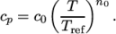
(7.8) - hPower
- calculates
 as a power of
temperature according to:
as a power of
temperature according to:
(7.9) - hTabulated
- calculates
 by interpolating
uniform tabulated data of
by interpolating
uniform tabulated data of  value pairs, e.g.:
( (200 1005) (400 1020) ); - janaf
- calculates
 as a function of
temperature
as a function of
temperature  from a set of coefficients taken from JANAF tables of thermodynamics. The ordered
list of coefficients is given in Table 7.1.
The function is valid between a lower and upper limit in
temperature
from a set of coefficients taken from JANAF tables of thermodynamics. The ordered
list of coefficients is given in Table 7.1.
The function is valid between a lower and upper limit in
temperature  and
and  respectively. Two sets of coefficients are specified,
the first set for temperatures above a common temperature
respectively. Two sets of coefficients are specified,
the first set for temperatures above a common temperature
 (and below
  ), the second for temperatures below
  (and above
  ). The function
relating
). The function
relating  to temperature is:
In addition, there are constants of integration,
(7.10)  and
and  , both at high and
low temperature, used to evaluating
, both at high and
low temperature, used to evaluating  and
and  respectively.


7.1.4 Composition of each constituent
There is currently only one option for the specie model which specifies the composition of each constituent. That model is itself named specie, which is specified by the following entries.
- nMoles: number of moles of component. This entry is only used for combustion modelling based on regress variable with a homogeneous mixture of reactants; otherwise it is set to 1.
- molWeight in grams per mole of specie.
7.1.5 Equation of state
The following equations of state are available in the thermophysical modelling library.
- adiabaticPerfectFluid
- Adiabatic perfect fluid:
where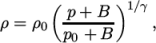
(7.11)  are reference density and pressure respectively, and
 is
a model constant.
is
a model constant. - Boussinesq
- Boussinesq approximation
where![ρ = ρ [1− β(T − T )] 0 0 \relax \special {t4ht=](img/index514x.png)
(7.12)  is the coeffient of volumetric expansion and
  is the reference
density at reference temperature
is the reference
density at reference temperature  .
. - icoPolynomial
- Incompressible, polynomial equation of
state:
where
(7.13)  are polynomial coefficients of any order
  .
. - icoTabulated
- Tabulated data for an incompressible fluid
using
 value pairs, e.g.
rho ( (200 1010) (400 980) ); - incompressiblePerfectGas
- Perfect gas for an incompressible fluid:
where
(7.14)  is a reference pressure.
 - linear
- Linear equation of state:
where
(7.15)  is compressibility (not necessarily
  ).
). - PengRobinsonGas
- Peng Robinson equation of state:
where the complex function
(7.16)  can be referenced in the source code in
PengRobinsonGasI.H, in the
$FOAM_SRC/thermophysicalModels/specie/equationOfState/
directory.
can be referenced in the source code in
PengRobinsonGasI.H, in the
$FOAM_SRC/thermophysicalModels/specie/equationOfState/
directory. - perfectFluid
- Perfect fluid:
where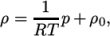
(7.17)  is the density at
  .
. - perfectGas
- Perfect gas:

(7.18) - rhoConst
- Constant density:

(7.19) - rhoTabulated
- Uniform tabulated data for a compressible
fluid, calculating
 as a function of
  and
and  .
. - rPolynomial
- Reciprocal polynomial equation of state for
liquids and solids:
where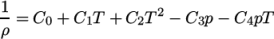
(7.20)  are coefficients.
7.1.6 Selection of energy variable
The user must
specify the form of energy to be used in the solution, either
internal energy  and enthalpy
  , and in forms that include the heat of
formation
, and in forms that include the heat of
formation  or not. This choice is specified through the energy keyword.
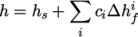
We refer to absolute energy where heat of formation is
included, and sensible energy
where it is not. For example absolute enthalpy  is related to sensible
enthalpy
is related to sensible
enthalpy  by
by
 |
(7.21) |
 and
and  are the molar fraction and heat of formation,
respectively, of specie
are the molar fraction and heat of formation,
respectively, of specie  . In most cases, we use the sensible form of
energy, for which it is easier to account for energy change due to
reactions. Keyword entries for energy therefore include e.g. sensibleEnthalpy, sensibleInternalEnergy and absoluteEnthalpy.
. In most cases, we use the sensible form of
energy, for which it is easier to account for energy change due to
reactions. Keyword entries for energy therefore include e.g. sensibleEnthalpy, sensibleInternalEnergy and absoluteEnthalpy.
7.1.7 Thermophysical property data
The basic thermophysical properties are specified for each species from input data. Data entries must contain the name of the specie as the keyword, e.g. O2, H2O, mixture, followed by sub-dictionaries of coefficients, including:
- specie
- containing i.e. number of moles, nMoles, of the specie, and molecular weight, molWeight in units of g/mol;
- thermodynamics
- containing coefficients for the chosen thermodynamic model (see below);
- transport
- containing coefficients for the chosen tranpsort model (see below).
The following is an example entry for a specie named fuel modelled using sutherland transport and janaf thermodynamics:
fuel
{
specie
{
nMoles 1;
molWeight 16.0428;
}
thermodynamics
{
Tlow 200;
Thigh 6000;
Tcommon 1000;
highCpCoeffs (1.63543 0.0100844 -3.36924e-06 5.34973e-10
-3.15528e-14 -10005.6 9.9937);
lowCpCoeffs (5.14988 -0.013671 4.91801e-05 -4.84744e-08
1.66694e-11 -10246.6 -4.64132);
}
transport
{
As 1.67212e-06;
Ts 170.672;
}
}
air
{
specie
{
nMoles 1;
molWeight 28.96;
}
thermodynamics
{
Cp 1004.5;
Hf 2.544e+06;
}
transport
{
mu 1.8e-05;
Pr 0.7;
}
}