Energy Equation in OpenFOAM

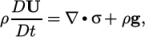
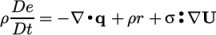
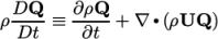
Contents

1 Introduction

This article provides information on the equation describing conservation of energy relevant to fluid dynamics and computational fluid dynamics (CFD). It first assembles an equation for combined mechanical and thermal energy, i.e. total energy, in terms of material derivatives. It then presents an equation for thermal, or internal, energy. The total energy equation is then provided in terms of local (partial) derivatives, both in terms of internal energy and enthalpy. The implementation of the energy equation in solvers in OpenFOAM is then described.

Some of the information in this article is also presented in the book Notes on CFD: General Principles.

2 Total Energy

The law of conservation of energy states that the total energy of an isolated system remains constant, i.e. it is conserved over time and energy is not created or destroyed but is transformed from one form to another. Here we consider only mechanical and thermodynamic energy, the contributions of which are described in the following sections, using usual notation of tensor algebra and calculus, including representing the material derivative.

2.1 Mechanical Power

The rate of change of mechanical, or kinetic, energy is:

(1)

where is velocity, specific kinetic energy (kinetic energy per unit mass) and is mass density. The power flux, or rate of change of strain energy, is

(2)

where is the mechanical stress tensor. The stress tensor may be decomposed into a scalar thermodynamic pressure and viscous stress tensor by , where is the identity tensor. The power source, or rate of change of potential energy, is

(3)

where is a body acceleration, e.g. gravity.

2.2 Thermodynamic Power

The rate of change of thermal, or internal, energy is

(4)

where is specific internal energy (internal energy per unit mass). The heat flux is

(5)

where is the heat flux vector, defined positive inwards. The heat source is

(6)

where is any specific heat source.

2.3 Conservation of Energy

The rate of change of total energy for a particle of material must equal the input of mechanical and thermodynamic power from fluxes and sources acting on the particle. In the limit where particle size is infinitesimally small

(7)

3 Internal Energy

An equation for internal energy is produced by simplifying the mechanical contributions which, expressed as

(8)

combines with the momentum equation

(9)

to reduce the mechanical contributions to . Equation 7 can then be expressed as

(10)

The term represents the contribution of mechanical power to internal energy, and thus, random motion of particles. The expression must then represent a power due bulk motion of particles.

4 Total Energy/Enthalpy, local derivatives

We can express our equations in terms of the local derivative (or partial derivative, spatial derivative, …) , where 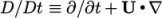. Applying conservation of mass, the following relationship holds for any tensor :

(11)

Combining equations 7 and 11, and decomposing the stress tensor , gives:

(12)

Enthalpy is the sum of internal energy and kinematic pressure, i.e. . Combining this with equation 12 gives:

(13)

Total energy can be defined as . Combining this with equation 12 gives:

(14)

5 Energy Equation in OpenFOAM Solvers

The solution of the energy equation is included in several solvers in OpenFOAM for compressible flow, combustion, heat transfer, multiphase flow and particle tracking. The source code can be found for these solvers within files in sub-directories of the $FOAM_SOLVERS directory of OpenFOAM (including the compressible, combustion, heatTransfer, multiphase and lagrangian sub-directories).

The energy equation is generally implemented in the form of total energy expressed in equations 12 and 13, without the mechanical sources and . A heat flux is assumed, where the effective thermal diffusivity is the sum of laminar and turbulent thermal diffusivities. The implementation of each energy equation contains thermal source terms relevant to the particular solver.

For example, the sonicFoam solver contains the following implementation of the energy equation from equation 12.

sonicFoam solves equations sequentially, so solves the momentum equation for before updating the specific kinetic energy field for the energy equation above. More commonly, the energy equation is implemented in terms of both internal energy and enthalpy , as both equations 12 and 13, allowing the user to choose the solution variable, or , at run time. For example, the rhoPimpleFoam solver has the following implementation:

Here, “he” represents either or . The 5th term switches between and depending on the solution variable chosen by the user.

The rhoCentralFoam solver includes an implementation of an energy equation best represented by equation 14 that includes the mechanical source .

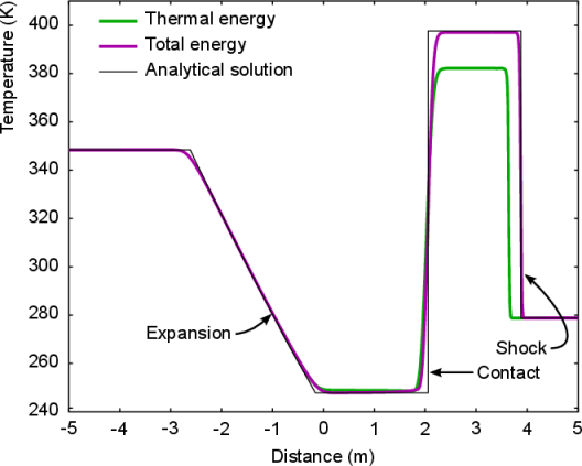
6 Total vs Internal Energy

The choice of energy equation has a significant on some solutions particularly across shocks. In the well known 1D shockTube tutorial example (Sod’s problem), the initial discontinuity causes a shock to propagate into the low pressure region and an expansion wave to propagate upstream. The figure below shows the temperature after 0.007 s, with simulation results compared with the analytical solution. Using the version of sonicFoam prior to OpenFOAM v2.2.0 that solves a thermal energy equation, the temperature difference across the shock is badly predicted. Using sonicFoam from v2.2.0 onwards that solves a total energy equation, conservation of total energy ensures the temperature difference is predicted accurately.

---

---