[version 14][version 13][version 12][version 11][version 10][version 9][version 8][version 7][version 6]
6.3 Sampling and monitoring data
There are a set of general post-processing functions for sampling data across the domain for graphs and visualisation. Several functions also provide data in a single file, in the form of time versus values, that can be plotted onto graphs. This time-value data can be monitored during a simulation with the foamMonitor script.
6.3.1 Probing data
The functions for probing data are boundaryProbes, internalProbes and probes as listed in section 6.2.1.11 . All functions work on the basis that the user provides some point locations and a list of fields, and the function writes out values of the fields are those locations. The differences between the functions are as follows.
- probes identifies the nearest cells to the probe locations and writes out the cell values; data is written into a single file in time-value format, suitable for plotting a graph.
- boundaryProbes and internalProbes interpolate field data to the probe locations, with the locations being snapped onto boundaries for boundaryProbes; data sets are written to separate files at scheduled write times (like fields). data.
Generally probes is more suitable for monitoring values at smaller numbers of locations, whereas the other functions are typically for sampling at large numbers of locations.
As an example, the user could use the pitzDaily case set up in section 6.2.3 . The probes function is best configured by copying the file to the local system directory using foamGet.
foamGet probes
13#includeEtc "caseDicts/postProcessing/probes/probes.cfg"
14
15fields (p U);
16probeLocations
17(
18 (0.01 0 0)
19);
20
21// ************************************************************************* //
The configuration is completed by adding the #includeFunc directive to functions in the controlDict file.
functions
{
#includeFunc probes
... other function objects here ...
}
6.3.2 Sampling for graphs
The graphUniform function samples data for graph plotting. To use it, the graphUniform file can be copied into the system directory to be configured. We will configure it here using the pitzDaily case as before. The file is simply copied using foamGet.
foamGet graphUniform
14start (0.01 0.025 0);
15end (0.01 -0.025 0);
16nPoints 100;
17
18fields (U p);
19
20axis distance; // The independent variable of the graph. Can be "x",
21 // "y", "z", "xyz" (all coordinates written out), or
22 // "distance" (from the start point).
23
24#includeEtc "caseDicts/postProcessing/graphs/graphUniform.cfg"
25
26// ************************************************************************* //
The configuration is completed by adding the #includeFunc directive to functions in the controlDict file.
functions
{
#includeFunc graphUniform
... other function objects here ...
}
 -component of velocity,
 in
the last time 296, by running
gnuplot and plotting values.
in
the last time 296, by running
gnuplot and plotting values.
gnuplot
gnuplot> set style data linespoints
gnuplot> plot "postProcessing/graphUniform/296/line_U.xy" u 2:1
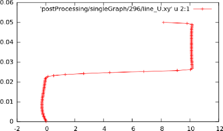
 at
at  = 0.01,
uniform sampling
= 0.01,
uniform samplingThe formatting of the graph is specified in configuration files in $FOAM_ETC/caseDicts/postProcessing/graphs. The graphUniform.cfg file in that directory includes the configuration as follows.
9#includeEtc "caseDicts/postProcessing/graphs/graph.cfg"
10
11sets
12(
13 line
14 {
15 type lineUniform;
16 axis $axis;
17 start $start;
18 end $end;
19 nPoints $nPoints;
20 }
21);
22
23// ************************************************************************* //
It shows that the sampling type is lineUniform, meaning the sampling uses a uniform distribution of points along a line. The other parameters are included by macro expansion from the main file and specify the line start and end, the number of points and the distance parameter specified on the horizontal axis of the graph.
An alternative graph function object, graphCell, samples the data at locations nearest to the cell centres. The user can copy that function object file and configure it as shown below.
14start (0.01 -0.025 0);
15end (0.01 0.025 0);
16fields (U p);
17
18axis distance; // The independent variable of the graph. Can be "x",
19 // "y", "z", "xyz" (all coordinates written out), or
20 // "distance" (from the start point).
21
22#includeEtc "caseDicts/postProcessing/graphs/graphCell.cfg"
23
24// ************************************************************************* //
Running simpleFoam produces the graph in Figure 6.6 .
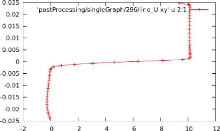
 at
at  = 0.01,
mid-point sampling
= 0.01,
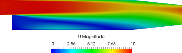
mid-point sampling6.3.3 Sampling for visualisation
There are several surfaces and streamlines functions, listed in Section 6.2.1.14 , that can be used to generate files for visualisation. The use of streamlinesLine is already configured in the pitzDaily case.
To generate a cutting plane, the cutPlaneSurface function can be configured by copying the cutPlaneSurface file to the system directory using foamGet.
foamGet cutPlaneSurface
 -direction.
17fields (p U);
18
19interpolate true; // If false, write cell data to the surface triangles.
20 // If true, write interpolated data at the surface points.
21
22#includeEtc "caseDicts/postProcessing/surface/cutPlaneSurface.cfg"
23
24// ************************************************************************* //
The function can be included as normal by adding the #includeFunc directive to functions in the controlDict file. Alternatively, the user could test running the function using the solver post-processing by the following command.
simpleFoam -postProcess -func cutPlaneSurface
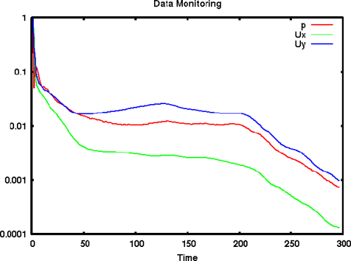
6.3.4 Live monitoring of data
Functions like probes produce a single file of time-value data, suitable for graph plotting. When the function is executed during a simulation, the user may wish to monitor the data live on screen. The foamMonitor script enables this; to discover its functionality, the user run it with the -help option. The help option includes an example of monitoring residuals that we can demonstrate in this section.
Firstly, include the residuals function in the controlDict file.
functions
{
#includeFunc residuals
... other function objects here ...
}
foamInfo residuals
foamGet residuals
It is advisable to delete the postProcessing directory to avoid duplicate files for each function. The user can delete the directory, then run simpleFoam in the background.
rm -rf postProcessing
simpleFoam > log &
 -axis on the
residuals file as follows. If
the command is executed before the simulation is complete, they can
see the graph being updated live.
-axis on the
residuals file as follows. If
the command is executed before the simulation is complete, they can
see the graph being updated live.
foamMonitor -l postProcessing/residuals/0/residuals.dat