[version 14][version 13][version 12][version 11][version 10][version 9][version 8][version 7][version 6]
2.3 Breaking of a dam
In this tutorial we shall solve a problem of simplified dam break in 2
dimensions using the interFoam.The feature of the problem is a transient
flow of two fluids separated by a sharp interface, or free surface. The
two-phase algorithm in interFoam is based on the volume of fluid (VOF)
method in which a specie transport equation is used to determine the
relative volume fraction of the two phases, or phase fraction  , in each
computational cell. Physical properties are calculated as weighted averages
based on this fraction. The nature of the VOF method means that an
interface between the species is not explicitly computed, but rather emerges
as a property of the phase fraction field. Since the phase fraction can
have any value between 0 and 1, the interface is never sharply defined,
but occupies a volume around the region where a sharp interface should
exist.
, in each
computational cell. Physical properties are calculated as weighted averages
based on this fraction. The nature of the VOF method means that an
interface between the species is not explicitly computed, but rather emerges
as a property of the phase fraction field. Since the phase fraction can
have any value between 0 and 1, the interface is never sharply defined,
but occupies a volume around the region where a sharp interface should
exist.
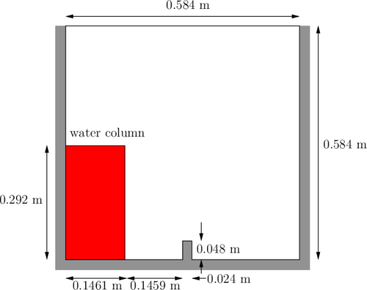
The test setup consists of a column of water at rest located behind a
membrane on the left side of a tank. At time  , the membrane is removed
and the column of water collapses. During the collapse, the water impacts an
obstacle at the bottom of the tank and creates a complicated flow structure,
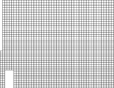
including several captured pockets of air. The geometry and the initial setup is
shown in Figure 2.21.
, the membrane is removed
and the column of water collapses. During the collapse, the water impacts an
obstacle at the bottom of the tank and creates a complicated flow structure,
including several captured pockets of air. The geometry and the initial setup is
shown in Figure 2.21.
2.3.1 Mesh generation
The user should go to their run directory and copy the damBreak case from the $FOAM_TUTORIALS/multiphase/interFoam/laminar/damBreak directory, i.e.
run
cp -r $FOAM_TUTORIALS/multiphase/interFoam/laminar/damBreak/damBreak .
18
19vertices
20(
21 (0 0 0)
22 (2 0 0)
23 (2.16438 0 0)
24 (4 0 0)
25 (0 0.32876 0)
26 (2 0.32876 0)
27 (2.16438 0.32876 0)
28 (4 0.32876 0)
29 (0 4 0)
30 (2 4 0)
31 (2.16438 4 0)
32 (4 4 0)
33 (0 0 0.1)
34 (2 0 0.1)
35 (2.16438 0 0.1)
36 (4 0 0.1)
37 (0 0.32876 0.1)
38 (2 0.32876 0.1)
39 (2.16438 0.32876 0.1)
40 (4 0.32876 0.1)
41 (0 4 0.1)
42 (2 4 0.1)
43 (2.16438 4 0.1)
44 (4 4 0.1)
45);
46
47blocks
48(
49 hex (0 1 5 4 12 13 17 16) (23 8 1) simpleGrading (1 1 1)
50 hex (2 3 7 6 14 15 19 18) (19 8 1) simpleGrading (1 1 1)
51 hex (4 5 9 8 16 17 21 20) (23 42 1) simpleGrading (1 1 1)
52 hex (5 6 10 9 17 18 22 21) (4 42 1) simpleGrading (1 1 1)
53 hex (6 7 11 10 18 19 23 22) (19 42 1) simpleGrading (1 1 1)
54);
55
56edges
57(
58);
59
60boundary
61(
62 leftWall
63 {
64 type wall;
65 faces
66 (
67 (0 12 16 4)
68 (4 16 20 8)
69 );
70 }
71 rightWall
72 {
73 type wall;
74 faces
75 (
76 (7 19 15 3)
77 (11 23 19 7)
78 );
79 }
80 lowerWall
81 {
82 type wall;
83 faces
84 (
85 (0 1 13 12)
86 (1 5 17 13)
87 (5 6 18 17)
88 (2 14 18 6)
89 (2 3 15 14)
90 );
91 }
92 atmosphere
93 {
94 type patch;
95 faces
96 (
97 (8 20 21 9)
98 (9 21 22 10)
99 (10 22 23 11)
100 );
101 }
102);
103
104mergePatchPairs
105(
106);
107
108// ************************************************************************* //
2.3.2 Boundary conditions
The user can examine the boundary geometry generated by blockMesh by viewing the boundary file in the constant/polyMesh directory. The file contains a list of 5 boundary patches: leftWall, rightWall, lowerWall, atmosphere and defaultFaces. The user should notice the type of the patches. The atmosphere is a standard patch, i.e. has no special attributes, merely an entity on which boundary conditions can be specified. The defaultFaces patch is empty since the patch normal is in the direction we will not solve in this 2D case. The leftWall, rightWall and lowerWall patches are each a wall.
Like the generic patch, the wall type contains no geometric or topological
information about the mesh and only differs from the plain patch in that it
identifies the patch as a wall, should an application need to know, e.g. to apply
special wall surface modelling. For example, the interFoam solver includes
modelling of surface tension and can include wall adhesion at the contact point
between the interface and wall surface. Wall adhesion models can be applied
through a special boundary condition on the alpha ( ) field, e.g. the
constantAlphaContactAngle boundary condition, which requires the user to specify
a static contact angle, theta0.
) field, e.g. the
constantAlphaContactAngle boundary condition, which requires the user to specify
a static contact angle, theta0.
In this tutorial we would like to ignore surface tension effects between the
wall and interface. We can do this by setting the static contact angle,
 . However, rather than using the constantAlphaContactAngle
boundary condition, the simpler zeroGradient can be applied to alpha on the
walls.
. However, rather than using the constantAlphaContactAngle
boundary condition, the simpler zeroGradient can be applied to alpha on the
walls.
The top boundary is free to the atmosphere so needs to permit both outflow and inflow according to the internal flow. We therefore use a combination of boundary conditions for pressure and velocity that does this while maintaining stability. They are:
- totalPressure which is a fixedValue condition calculated from specified total pressure p0 and local velocity U;
- pressureInletOutletVelocity, which applies zeroGradient on all components, except where there is inflow, in which case a fixedValue condition is applied to the tangential component;
- inletOutlet, which is a zeroGradient condition when flow outwards, fixedValue when flow is inwards.
At all wall boundaries, the fixedFluxPressure boundary condition is applied to the pressure field, which adjusts the pressure gradient so that the boundary flux matches the velocity boundary condition for solvers that include body forces such as gravity and surface tension.
The defaultFaces patch representing the front and back planes of the 2D problem, is, as usual, an empty type.
2.3.3 Setting initial field
Unlike the previous cases, we shall now specify a non-uniform initial condition for
the phase fraction  where
where
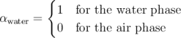 | (2.15) |
18defaultFieldValues
19(
20 volScalarFieldValue alpha.water 0
21);
22
23regions
24(
25 boxToCell
26 {
27 box (0 0 -1) (0.1461 0.292 1);
28 fieldValues
29 (
30 volScalarFieldValue alpha.water 1
31 );
32 }
33);
34
35
36// ************************************************************************* //
The defaultFieldValues sets the default value of the fields, i.e. the value the
field takes unless specified otherwise in the regions sub-dictionary. That
sub-dictionary contains a list of subdictionaries containing fieldValues that
override the defaults in a specified region. The region creates a set of points, cells
or faces based on some topological constraint. Here, boxToCell creates a
bounding box within a vector minimum and maximum to define the set of cells
of the water region. The phase fraction  is defined as 1 in this
region.
is defined as 1 in this
region.
The setFields utility reads fields from file and, after re-calculating those fields, will write them back to file. In the damBreak tutorial, the alpha.water field is initially stored as a backup named alpha.water.orig. A field file with the .orig extension is read in when the actual file does not exist, so setFields will read alpha.water.orig but write the resulting output to alpha.water (or alpha.water.gz if compression is switched on). This way the original file is not overwritten, so can be reused.
The user should therefore execute setFields like any other utility by:
setFields
2.3.4 Fluid properties
Let us examine the transportProperties file in the constant directory. The dictionary first contains the names of each fluid phase in the phases list, here water and air. The material properties for each fluid are then separated into two dictionaries water and air. The transport model for each phase is selected by the transportModel keyword. The user should select Newtonian in which case the kinematic viscosity is single valued and specified under the keyword nu. The viscosity parameters for other models, e.g.CrossPowerLaw, would otherwise be specified as described in section 7.3. The density is specified under the keyword rho.
The surface tension between the two phases is specified by the keyword sigma. The values used in this tutorial are listed in Table 2.3.
| water properties
| |||
| Kinematic viscosity |  | nu |  |
| Density |  | rho |  |
| air properties
| |||
| Kinematic viscosity |  | nu |  |
| Density |  | rho | 1.0 |
| Properties of both phases
| |||
| Surface tension |  | sigma | 0.07 |
Gravitational acceleration is uniform across the domain and is specified in a
file named g in the constant directory. Unlike a normal field file, e.g. U
and p, g is a uniformDimensionedVectorField and so simply contains a set
of dimensions and a value that represents 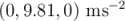 for this
tutorial:
for this
tutorial:
18dimensions [0 1 -2 0 0 0 0];
19value (0 -9.81 0);
20
21
22// ************************************************************************* //
2.3.5 Turbulence modelling
As in the cavity example, the choice of turbulence modelling method is selectable at run-time through the simulationType keyword in turbulenceProperties dictionary. In this example, we wish to run without turbulence modelling so we set laminar:
18simulationType laminar;
19
20
21// ************************************************************************* //
2.3.6 Time step control
Time step control is an important issue in transient simulation and the
surface-tracking algorithm in interface capturing solvers. The Courant number
 needs to be limited depending on the choice of algorithm: with the “explicit”
MULES algorithm, an upper limit of
needs to be limited depending on the choice of algorithm: with the “explicit”
MULES algorithm, an upper limit of  for stability is typical in the
region of the interface; but with “semi-implicit” MULES, specified by the
MULESCorr keyword in the fvSolution file, there is really no upper limit in for
stability, but instead the level is determined by requirements of temporal
accuracy.
for stability is typical in the
region of the interface; but with “semi-implicit” MULES, specified by the
MULESCorr keyword in the fvSolution file, there is really no upper limit in for
stability, but instead the level is determined by requirements of temporal
accuracy.
In general it is difficult to specify a fixed time-step to satisfy the  criterion, so interFoam offers automatic adjustment of the time step as
standard in the controlDict. The user should specify adjustTimeStep to be
on and the the maximum for the phase fields, maxAlphaCo, and
other fields, maxCo, to be 1.0. The upper limit on time step maxDeltaT
can be set to a value that will not be exceeded in this simulation, e.g.
1.0.
criterion, so interFoam offers automatic adjustment of the time step as
standard in the controlDict. The user should specify adjustTimeStep to be
on and the the maximum for the phase fields, maxAlphaCo, and
other fields, maxCo, to be 1.0. The upper limit on time step maxDeltaT
can be set to a value that will not be exceeded in this simulation, e.g.
1.0.
By using automatic time step control, the steps themselves are never rounded to a convenient value. Consequently if we request that OpenFOAM saves results at a fixed number of time step intervals, the times at which results are saved are somewhat arbitrary. However even with automatic time step adjustment, OpenFOAM allows the user to specify that results are written at fixed times; in this case OpenFOAM forces the automatic time stepping procedure to adjust time steps so that it ‘hits’ on the exact times specified for write output. The user selects this with the adjustableRunTime option for writeControl in the controlDict dictionary. The controlDict dictionary entries should be:
18application interFoam;
19
20startFrom startTime;
21
22startTime 0;
23
24stopAt endTime;
25
26endTime 1;
27
28deltaT 0.001;
29
30writeControl adjustableRunTime;
31
32writeInterval 0.05;
33
34purgeWrite 0;
35
36writeFormat binary;
37
38writePrecision 6;
39
40writeCompression off;
41
42timeFormat general;
43
44timePrecision 6;
45
46runTimeModifiable yes;
47
48adjustTimeStep yes;
49
50maxCo 1;
51maxAlphaCo 1;
52
53maxDeltaT 1;
54
55
56// ************************************************************************* //
2.3.7 Discretisation schemes
The interFoam solver uses the multidimensional universal limiter for explicit solution (MULES) method, created by Henry Weller, to maintain boundedness of the phase fraction independent of underlying numerical scheme, mesh structure, etc. The choice of schemes for convection are therfore not restricted to those that are strongly stable or bounded, e.g. upwind differencing.
The convection schemes settings are made in the divSchemes sub-dictionary of
the fvSchemes dictionary. In this example, the convection term in the momentum
equation ( ), denoted by the div(rhoPhi,U) keyword, uses Gauss
linearUpwind grad(U) to produce good accuracy. Here, we have opted for
best stability with
), denoted by the div(rhoPhi,U) keyword, uses Gauss
linearUpwind grad(U) to produce good accuracy. Here, we have opted for
best stability with  . The
. The  term, represented by the
div(phi,alpha) keyword uses the vanLeer scheme. The
term, represented by the
div(phi,alpha) keyword uses the vanLeer scheme. The  term,
represented by the div(phirb,alpha) keyword, can use second order
linear (central) differencing as boundedness is assured by the MULES
algorithm.
term,
represented by the div(phirb,alpha) keyword, can use second order
linear (central) differencing as boundedness is assured by the MULES
algorithm.
The other discretised terms use commonly employed schemes so that the fvSchemes dictionary entries should therefore be:
18ddtSchemes
19{
20 default Euler;
21}
22
23gradSchemes
24{
25 default Gauss linear;
26}
27
28divSchemes
29{
30 div(rhoPhi,U) Gauss linearUpwind grad(U);
31 div(phi,alpha) Gauss vanLeer;
32 div(phirb,alpha) Gauss linear;
33 div(((rho*nuEff)*dev2(T(grad(U))))) Gauss linear;
34}
35
36laplacianSchemes
37{
38 default Gauss linear corrected;
39}
40
41interpolationSchemes
42{
43 default linear;
44}
45
46snGradSchemes
47{
48 default corrected;
49}
50
51
52// ************************************************************************* //
2.3.8 Linear-solver control
In the fvSolution file, the alpha.water sub-dictionary in solvers contains
elements that are specific to interFoam. Of particular interest are the
nAlphaSubCycles and cAlpha keywords. nAlphaSubCycles represents the
number of sub-cycles within the  equation; sub-cycles are additional solutions
to an equation within a given time step. It is used to enable the solution
to be stable without reducing the time step and vastly increasing the
solution time. Here we specify 2 sub-cycles, which means that the
equation is solved in
equation; sub-cycles are additional solutions
to an equation within a given time step. It is used to enable the solution
to be stable without reducing the time step and vastly increasing the
solution time. Here we specify 2 sub-cycles, which means that the
equation is solved in  half length time steps within each actual time
step.
half length time steps within each actual time
step.
The cAlpha keyword is a factor that controls the compression of the interface where: 0 corresponds to no compression; 1 corresponds to conservative compression; and, anything larger than 1, relates to enhanced compression of the interface. We generally adopt a value of 1.0 which is employed in this example.
2.3.9 Running the code
Running of the code has been described in detail in previous tutorials. Try the following, that uses tee, a command that enables output to be written to both standard output and files:
cd $FOAM_RUN/damBreak
interFoam | tee log
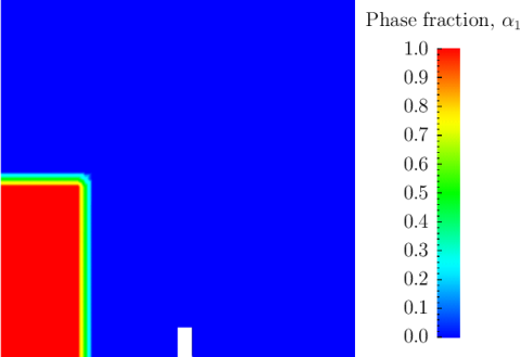
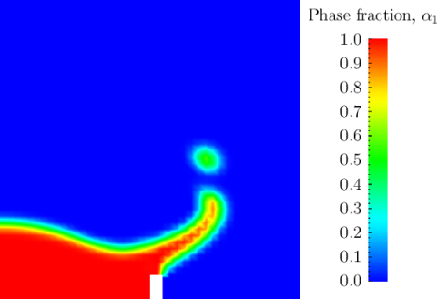
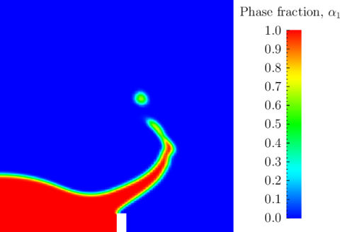
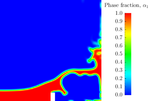
2.3.10 Post-processing
Post-processing of the results can now be done in the usual way. The user can monitor the development of the phase fraction alpha.water in time, e.g. see Figure 2.23.


 .
.2.3.11 Running in parallel
The results from the previous example are generated using a fairly coarse mesh. We now wish to increase the mesh resolution and re-run the case. The new case will typically take a few hours to run with a single processor so, should the user have access to multiple processors, we can demonstrate the parallel processing capability of OpenFOAM.
The user should first clone the damBreak case, e.g. by
run
foamCloneCase damBreak damBreakFine
blocks
(
hex (0 1 5 4 12 13 17 16) (46 10 1) simpleGrading (1 1 1)
hex (2 3 7 6 14 15 19 18) (40 10 1) simpleGrading (1 1 1)
hex (4 5 9 8 16 17 21 20) (46 76 1) simpleGrading (1 2 1)
hex (5 6 10 9 17 18 22 21) (4 76 1) simpleGrading (1 2 1)
hex (6 7 11 10 18 19 23 22) (40 76 1) simpleGrading (1 2 1)
);
As the mesh has now changed from the damBreak example, the user must
re-initialise the phase field alpha.water in the 0 time directory since it contains a
number of elements that is inconsistent with the new mesh. Note that there is no
need to change the U and p_rgh fields since they are specified as uniform which is
independent of the number of elements in the field. We wish to initialise
the field with a sharp interface, i.e. it elements would have  or
or
 . Updating the field with mapFields may produce interpolated
values
. Updating the field with mapFields may produce interpolated
values  at the interface, so it is better to rerun the setFields
utility.
at the interface, so it is better to rerun the setFields
utility.
The mesh size is now inconsistent with the number of elements in the alpha.water.gz file in the 0 directory, so the user must delete that file so that the original alpha.water.orig file is used instead.
rm 0/alpha.water.gz
setFields
The method of parallel computing used by OpenFOAM is known as domain decomposition, in which the geometry and associated fields are broken into pieces and allocated to separate processors for solution. The first step required to run a parallel case is therefore to decompose the domain using the decomposePar utility. There is a dictionary associated with decomposePar named decomposeParDict which is located in the system directory of the tutorial case; also, like with many utilities, a default dictionary can be found in the directory of the source code of the specific utility, i.e. in $FOAM_UTILITIES/parallelProcessing/decomposePar for this case.
The first entry is numberOfSubdomains which specifies the number of subdomains into which the case will be decomposed, usually corresponding to the number of processors available for the case.
In this tutorial, the method of decomposition should be simple and the
corresponding simpleCoeffs should be edited according to the following criteria.
The domain is split into pieces, or subdomains, in the  ,
,  and
and  directions,
the number of subdomains in each direction being given by the vector
directions,
the number of subdomains in each direction being given by the vector  . As
this geometry is 2 dimensional, the 3rd direction, , cannot be split,
hence
. As
this geometry is 2 dimensional, the 3rd direction, , cannot be split,
hence  must equal 1. The
  and
and  components of
  split the
domain in the
split the
domain in the  and
and  directions and must be specified so that the
number of subdomains specified by
directions and must be specified so that the
number of subdomains specified by  and
and  equals the specified
numberOfSubdomains, i.e.
equals the specified
numberOfSubdomains, i.e.  numberOfSubdomains. It is beneficial to keep
the number of cell faces adjoining the subdomains to a minimum so, for
a square geometry, it is best to keep the split between the
numberOfSubdomains. It is beneficial to keep
the number of cell faces adjoining the subdomains to a minimum so, for
a square geometry, it is best to keep the split between the  and
and  directions should be fairly even. The delta keyword should be set to
0.001.
directions should be fairly even. The delta keyword should be set to
0.001.
For example, let us assume we wish to run on 4 processors. We would set
numberOfSubdomains to 4 and  . The user should run decomposePar
with:
. The user should run decomposePar
with:
decomposePar
The user should consult section 3.4 for details of how to run a case in parallel; in this tutorial we merely present an example of running in parallel. We use the openMPI implementation of the standard message-passing interface (MPI). As a test here, the user can run in parallel on a single node, the local host only, by typing:
mpirun -np 4 interFoam -parallel > log &
The user may run on more nodes over a network by creating a file that lists the host names of the machines on which the case is to be run as described in section 3.4.3. The case should run in the background and the user can follow its progress by monitoring the log file as usual.


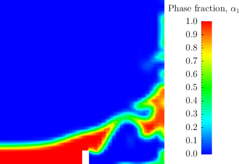
 with refined mesh.
2.3.12 Post-processing a case run in parallel
Once the case has completed running, the decomposed fields and mesh can be reassembled for post-processing using the reconstructPar utility. Simply execute it from the command line. The results from the fine mesh are shown in Figure 2.25. The user can see that the resolution of interface has improved significantly compared to the coarse mesh.
The user may also post-process an individual region of the decomposed domain individually by simply treating the individual processor directory as a case in its own right. For example if the user starts paraFoam by
paraFoam -case processor1