OpenFOAM v14 User Guide - 6.1 Field functions

6.1 Field functions

In the configuration of a CFD simulation, it is quite common for some fields to be initialised with an internalField that is nonuniform. Similarly in the boundaryField, initial values on the faces of some patches may also need to be nonuniform. There are many examples, where the initialisation of nonuniform fields is required, but a very common example occurs in multiphase flows where the initial phase fraction field, e.g. alpha.water, determines the position of the phase interface, and with it, the height of the liquid phase.

Prior to OpenFOAM v14, nonuniform fields were created firstly by configuring a uniform field, e.g. with alpha.water = 0 corresponding to “all air”. Then a pre-processing utility, typically setFields, would need to be configured and executed. It would read the initial uniform field, modify it and write out a new nonuniform field. Usually the initial field file would be created using the .orig extension, e.g. alpha.water.orig, so that it would not be overwritten (and thus, deleted) when the generated nonuniform field was written using conventional name alpha.water.

In OpenFOAM v14 however, field functions have been introduced that initialise nonuniform fields directly within the field files. This “local” initialisation is more self-contained, avoids the need to run a pre-processing utility, and offers more options to specify the initialisation up to even the most complex functions.

Field functions are specified for an internalField by replacing the uniform/nonuniform keyword in the usual syntax, e.g.

with a sub-dictionary entry that begins with the type keyword that specifies the choice of field function, e.g. There are six general field function that can be selected, listed below.

• zonal: field values are specified in different zones of the mesh.

• surfaces: field values are specified in different regions of mesh, separated by surfaces, e.g. searchable surfaces, STL/OBJ files, etc.

• coded: field values are defined by some code which is dynamically compiled.

• distanceFunction: field values are calculated using a Function1 of distance across the domain.

• fieldFunction: field values are calculated using a Function1 of another field, e.g. a function of the temperature field T.

• timeFunction: field values are calculated using a Function1 of time.

The following sections explain the use of each field function, with examples.

6.1.1 The zonal field function

The zonal field function is illustrated by the $FOAM_TUTORIALS/shockFluid/shockTube 1D example case. The 0/p file is initialised with  bar for and  bar for . The configuration of the internalField is as follows.

This works by first setting the defaultValue of the field to 1 bar. A cell zone is then created, named lowPressure, using a box zoneGenerator, which bounds the region of the mesh . Within the lowPressure zone, the pressure is set to 0.1 bar.

6.1.2 The surfaces field function

The $FOAM_TUTORIALS/compressibleVoF/depthCharge3D example case demonstrates the of the surfaces field function. In the case this field function initialises the phase fraction field in the 0/alpha.water file. It does so by initially setting the defaultValue to 1, i.e. to the water phase, before overriding the value to 0 to represent air both above an air-water interface and inside a bubble within the water region. The configuration of the internalField is as follows.

The plane surface is an infinite plane, positioned at  m and with its normal in the -direction. Since normal vectors conventionally point out of a surface, the notional “inside” is above the surface at  m, which is set to a value of 0, representing air.

The sphere surface represents a sphere, defined by the centre and radius. Inside the sphere the value is 0, representing an air bubble, as shown in Figure 6.1 .

---

---

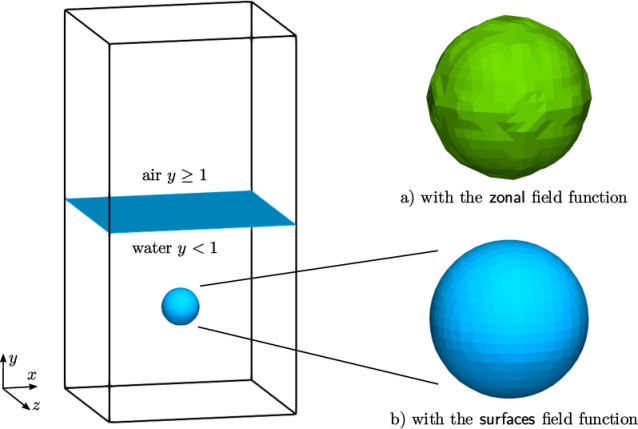
The surfaces field function performs cell cutting and calculates intermediate values in the cut cells. Cells intersected by the sphere surface therefore have intermediate values between 0 and 1. Consequently, the air-water interface, visualised by an iso-surface of alpha.water = 0.5, appears smooth as in Figure 6.1 b).

The zonal field function, by contrast, does not perform surface cutting. If it were to initialise the bubble with a sphere zone, the values of alpha.water would be either 0 or 1, depending on whether a given cell is inside the zone or not. Without intermediate values in around the interface, the iso-surface appears rough in Figure 6.1 a). Evidently the initialisation with the surfaces field function is more accurate than using zonal.

6.1.3 The coded field function

The coded field function allows the user to write code to describe the initial distribution of a field. This provides complete flexibility in initialising a field but can naturally be more complex than other options. So before attempting to use the coded field function, it is recommended to check whether one of the other options will work.

If the initialisation is not zonal in nature, the zonal and surfaces field functions are unlikely to be useful. Other than coded, all the remaining field function use a Function1 to describe the distribution. Function1 provides a wide range of pre-defined functions of one variable, discussed in section 6.4.4 , where the “one variable” is distance across the domain, time and another field for the distanceFunction, timeFunction and fieldFunction field functions, respectively.

If none of those field functions are suitable, the coded is likely the best option. One potential starting point for configuring such a field function is the $FOAM_TUTORIALS/incompressibleFluid/pipeCyclic example case. The case uses a quarter section of a pipe to demonstrate the behaviour of the cyclic patch types. To encourage the fluid through the cyclic patch, a swirl flow is applied at the inlet patch and also the internalField is initialised with the same swirl flow, as shown in Figure 6.2 .

---

---

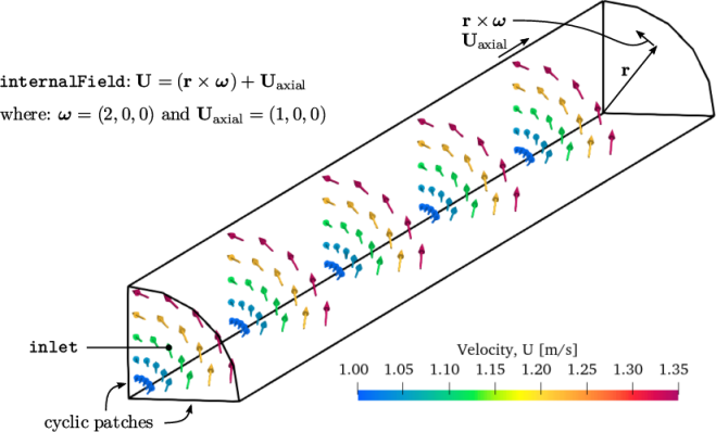
The swirl flow is defined by

(6.1)

where m s is the axial velocity, rad s is the rotational speed and is the position vector.

The coded field function is implemented in for internalField in the 0/U file. It includes a remarkably compact piece of code that represents Equation 6.1 using OpenFOAM’s equation syntax that includes ‘^’ to denote the cross product ().

Within the coded framework, there are two code block that can be defined.

• evaluate #{…#}; to initialise the field at the beginning of the simulation.

• update #{…#}; to update the field each time step during the simulation.

In the example, only the former is defined since the field is only initialised and requires no subsequent update during the simulation. To make code implementation easier the coded framework providing the following references.

• field: reference to the dimensionedField, which includes the internalField and dimensions.

• C: the cell centre vectors, also a dimensionedField, denoting ‘position’ in the domain.

• t: the time, as a dimensionedScalar.

In the code, therefore, the user can calculate any function of position and time assign the result to the field with field = … Calculations, and the assignment, include dimensions so are checked for dimensional consistency.

Consequently, the code generally requires parameters to be defined with dimensions. Often there are single valued parameters with dimensions, i.e. dimensioned values. The dimensionSet element can be specified using named dimensions — whose names are listed by running foamUnits, e.g. velocity, kinematicViscosity, etc. These names exist within a dimensions namespace in OpenFOAM, so would normally be specified with the qualifier, e.g. dimensions::velocity. However, the coded framework includes the directive

so the named dimensions do not require a qualifier, i.e. “velocity” is sufficient to specify the dimensions of velocity in the code. The dimensioned parameter for velocity would then normally be constructed as follows: To simplify this code, OpenFOAM v14 includes a variadic template function to create a dimensioned parameter using the syntax where components cmpt0, etc. can include any number of components for scalar, vector, tensor, etc. For example, for a vector with 3 components and dimensions of velocity, the code combines the velocity dimensions with the 3 components of the vector, as follows. In addition to the specific “hooks”, i.e. the field, C and t, a coded field function can include any OpenFOAM code to perform the calculations required. For example, the mesh and its data can be accessed directly from the field reference, by calling the standard mesh() access function with field.mesh(). The user therefore has complete freedom to initialise a field within the limits of the knowledge and skill of programming with OpenFOAM.

6.1.4 The distanceFunction field function

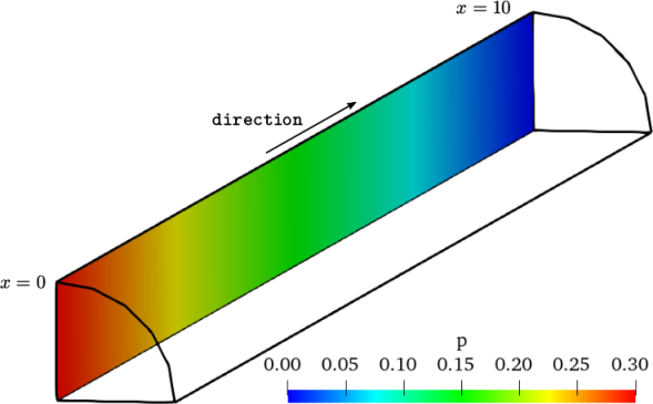
The distanceFunction is the first of the field functions where the initialisation is performed using a Function1. As mentioned earlier, Function1 provides a wide range of pre-defined functions of one variable, described in section 6.4.4 . In this case the variable is distance across the domain. An example of a distanceFunction is shown below.

This field function requires a direction entry to define the direction in which the distance function variable is defined. Specifically, the function variable is , where is the position vector for cell centres and is the unit direction vector. The distance variable is therefore the -ordinate of the position.

The function entry then contains the specification of a Function1. The example uses a table function with two value pairs. The entries specify a value of 0.3 at (the distance variable here) and a value of 0 at , with table data interpolated linearly at points between value pairs.

Applying this field function the internalField in 0/p in the previous example case, gives the initialisation of pressure as shown in Figure 6.3.

---

---

6.1.5 The fieldFunction field function

An example of the fieldFunction field function is provided in the $FOAM_TUTORIALS/multiRegion/CHT/hotWire case. In that case, the field function is used to specify a field used in an fvModel for calculating electrical conduction.

The field concerned is sigma, denoting electrical conductivity , which varies as a function of temperature . Since varies with time, the field also varies in time. Similarly, for the timeFunction field function in the following section, the field varies over time. Inevitably time-varying fields tend to appear in models, configured in the fvModels file, rather than as fields in the 0 directory, which are generally modified as part of the solution of governing equations.

The field function for sigma is in the constant/fvModels file within the solidElectricalConduction model and is reproduced below.

It uses the polynomial Function1, as a function of , meaning the applied function is .

6.1.6 The timeFunction field function

The timeFunction function object is applied similarly to fieldFunction above. If, for example, a user wished to prescribe an electrical conductivity field which varies as a prescribed function of time , then timeFunction would be suitable. A hypothetical configuration, similar to that of the fieldFunction above, is given as follows.

This would represent a function .

6.1.7 Applied field functions

As stated in the introduction to section 6.1 , direct initialisation of field files with field functions largely replaces running pre-processing utilities, e.g. setFields, to initialise fields. As well as setFields, there are some bespoke pre-processing utilities to initialise fields for specific applications. In particular: the setAtmBoundaryLayer utility initialises fields corresponding to the velocity profile of an an atmospheric boundary layer; and, the setWaves utility initialises surface waves in a liquid.

In OpenFOAM v14, both these utilities can be replaced using bespoke field functions. For an atmospheric boundary layer, there are atmosphericBoundaryLayerVelocity, atmosphericBoundaryLayerTurbulentKineticEnergy and atmosphericBoundaryLayerEpsilon field functions to initialise the U, k and epsilon fields, respectively. For surface waves, the waveAlpha and waveVelocity field functions to initialise the phase fraction field, e.g. alpha.water, and the U field, respectively.

These field functions read their configuration file, atmosphericBoundaryLayerProperties or waveProperties, from the constant directory. They use the parameters from the file to construct the distribution of their respective field; since the configuration of the parameters is in a separate file, the syntax within a field file itself is very compact, e.g. as follows for 0/U.

The libs entry above loads the relevant library containing the field function. If in doubt, running foamToC with the -search option will provide the library name. Example cases that include an atmospheric boundary layer and those that include surface waves can be located using foamFind as follows. The field functions for atmospheric boundary layers and surface waves have equivalent boundary conditions of the same name. These are inlet-outlet type conditions that specify a fixed value for inflow using the values prescribed by the field function, and zero gradient for outflow.

The syntax for specifying the field function and the boundary condition are the same, so the boundary condition can be specified using a macro expansion of the internalField keyword. For a patch named inlet, the syntax would be as follows.