[version 13][version 12][version 11][version 10][version 9][version 8][version 7][version 6]
2.2 Breaking of a dam
In this example we shall solve a problem of a
simplified dam break in 2 dimensions using the incompressibleVoF modular solver. The feature of the problem is a
transient flow of two fluids separated by a sharp interface, or free
surface. The two-phase algorithm in
incompressibleVoF is based on
the volume of fluid (VoF) method in which a phase transport equation
is used to determine the relative volume fraction of the two
phases, or phase fraction  , in each computational cell. Physical
properties are calculated as weighted averages based on this
fraction. The nature of the VoF method means that an interface
between the phases is not explicitly computed, but rather emerges
as a property of the phase fraction field. Since the phase fraction
can have any value between 0 and 1, the interface is never
precisely defined, but occupies a volume around the region where a
sharp interface should exist.
, in each computational cell. Physical
properties are calculated as weighted averages based on this
fraction. The nature of the VoF method means that an interface
between the phases is not explicitly computed, but rather emerges
as a property of the phase fraction field. Since the phase fraction
can have any value between 0 and 1, the interface is never
precisely defined, but occupies a volume around the region where a
sharp interface should exist.
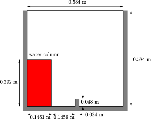
The test setup consists of a column of water at
rest located behind a membrane on the left side of a tank. At time
 ,
the membrane is removed and the column of water collapses. During
the collapse, the water impacts an obstacle at the bottom of the
tank and creates a complicated flow structure, including several
captured pockets of air. The geometry and the initial setup is
shown in Figure 2.15
.
,
the membrane is removed and the column of water collapses. During
the collapse, the water impacts an obstacle at the bottom of the
tank and creates a complicated flow structure, including several
captured pockets of air. The geometry and the initial setup is
shown in Figure 2.15
.
2.2.1 Mesh generation
The user should go to their run directory and copy the damBreakLaminar case from the $FOAM_TUTORIALS/incompressibleVoF directory, i.e.
run
cp -r $FOAM_TUTORIALS/incompressibleVoF/damBreakLaminar .
16convertToMeters 0.146;

17

18vertices

19(

20    (0 0 0)

21    (2 0 0)

22    (2.16438 0 0)

23    (4 0 0)

24    (0 0.32876 0)

25    (2 0.32876 0)

26    (2.16438 0.32876 0)

27    (4 0.32876 0)

28    (0 4 0)

29    (2 4 0)

30    (2.16438 4 0)

31    (4 4 0)

32    (0 0 0.1)

33    (2 0 0.1)

34    (2.16438 0 0.1)

35    (4 0 0.1)

36    (0 0.32876 0.1)

37    (2 0.32876 0.1)

38    (2.16438 0.32876 0.1)

39    (4 0.32876 0.1)

40    (0 4 0.1)

41    (2 4 0.1)

42    (2.16438 4 0.1)

43    (4 4 0.1)

44);

45

46blocks

47(

48    hex (0 1 5 4 12 13 17 16) (23 8 1) simpleGrading (1 1 1)

49    hex (2 3 7 6 14 15 19 18) (19 8 1) simpleGrading (1 1 1)

50    hex (4 5 9 8 16 17 21 20) (23 42 1) simpleGrading (1 1 1)

51    hex (5 6 10 9 17 18 22 21) (4 42 1) simpleGrading (1 1 1)

52    hex (6 7 11 10 18 19 23 22) (19 42 1) simpleGrading (1 1 1)

53);

54

55defaultPatch

56{

57    type empty;

58}

59

60boundary

61(

62    leftWall

63    {

64        type wall;

65        faces

66        (

67            (0 12 16 4)

68            (4 16 20 8)

69        );

70    }

71    rightWall

72    {

73        type wall;

74        faces

75        (

76            (7 19 15 3)

77            (11 23 19 7)

78        );

79    }

80    lowerWall

81    {

82        type wall;

83        faces

84        (

85            (0 1 13 12)

86            (1 5 17 13)

87            (5 6 18 17)

88            (2 14 18 6)

89            (2 3 15 14)

90        );

91    }

92    atmosphere

93    {

94        type patch;

95        faces

96        (

97            (8 20 21 9)

98            (9 21 22 10)

99            (10 22 23 11)

100        );

101    }

102);

103

104

105// ************************************************************************* //
The mesh is written into a set of files in a polyMesh directory in the constant directory. The user can list the contents of the directory to reveal the set of files/
ls constant/polyMesh
2.2.2 Boundary conditions
The boundary file can be read and understood by the user. The user should take a look at its contents, either by opening it in a file editor or printing out in the terminal window using the cat utility.
cat constant/polyMesh/boundary
The leftWall, rightWall and lowerWall patches are each a wall. Like the generic patch, the wall type contains no geometric or topological information about the mesh and only differs from the plain patch in that it identifies the patch as a wall. This is required by some modelling, e.g. turbulent wall functions and some turbulence models which include the distance to the nearest wall in their calculations.
With VoF specifically, surface tension models can
include wall adhesion at the contact point between the interface
and wall surface. Wall adhesion models can be applied through a
special boundary condition on the alpha ( ) field, e.g. the alphaContactAngle boundary condition, which
requires the user to specify a static contact angle, theta0.
) field, e.g. the alphaContactAngle boundary condition, which
requires the user to specify a static contact angle, theta0.
This example ignores surface tension effects
between the wall and interface. This can be done can do this by
setting the static contact angle,  , but a simpler approach
is to apply the zeroGradient
condition to alpha on the
walls.
, but a simpler approach
is to apply the zeroGradient
condition to alpha on the
walls.
The top boundary is free to the atmosphere so needs to permit both outflow and inflow according to the internal flow. We therefore use a combination of boundary conditions for pressure and velocity that does this while maintaining stability. They are:
-
prghTotalPressure, applied to the pressure field, minus the hydrostatic component,
 , given by
Equation 6.4
;
, given by
Equation 6.4
; -
pressureInletOutletVelocity, applied to velocity
 , which sets zeroGradient on all components of
,
except where there is inflow, in which case a fixedValue condition is applied to the
tangential component;
, which sets zeroGradient on all components of
,
except where there is inflow, in which case a fixedValue condition is applied to the
tangential component; -
inletOutlet applied to other fields, which is a zeroGradient condition when flow outwards, fixedValue when flow is inwards.
At all wall boundaries, the fixedFluxPressure boundary condition is applied to the pressure field, which adjusts the pressure gradient so that the boundary flux matches the velocity boundary condition for solvers that include body forces such as gravity and surface tension.
The defaultFaces patch representing the front and back planes of the 2D problem, is, as usual, an empty type.
2.2.3 Phases
The fluid phases are specified in the phaseProperties file in the constant directory as follows:
16

17phases          (water air);

18

19sigma           0.07;

20

21

22// ************************************************************************* //
It lists two phases, water and air. Equations for phase fraction are
solved for the phases in the list, except the last phase listed, i.e. air in this case. Since there are only two
phases, only one phase fraction equation is solved in this case,
for the water phase fraction  , specified in the file
alpha.water in the
0 directory.
, specified in the file
alpha.water in the
0 directory.
The phaseProperties file also contains an entry
for the surface tension between the two phases, specified by the
keyword sigma in units  .
.
2.2.4 Setting initial fields
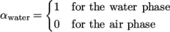
Unlike the previous cases, we shall now specify
a non-uniform initial condition for the phase fraction  where
where
 |
(2.5) |
16

17defaultFieldValues

18(

19    volScalarFieldValue alpha.water 0

20    volScalarFieldValue tracer.water 0

21    volScalarFieldValue tracer.air 0

22);

23

24regions

25(

26    boxToCell

27    {

28        box (0 0 -1) (0.1461 0.292 1);

29        fieldValues

30        (

31            volScalarFieldValue alpha.water 1

32        );

33    }

34    boxToCell

35    {

36        box (0 0 -1) (0.1461 0.146 1);

37        fieldValues

38        (

39            volScalarFieldValue tracer.water 1

40        );

41    }

42    boxToCell

43    {

44        box (0 0.292 -1) (0.1461 0.438 1);

45        fieldValues

46        (

47            volScalarFieldValue tracer.air 1

48        );

49    }

50);

51

52

53// ************************************************************************* //
The defaultFieldValues sets the default value of
the fields, i.e. the value the
field takes unless specified otherwise in the regions list. That list contains sub-dictionaries with
fieldValues that override the defaults
in a specified region. Regions are defined by functions that define a
set of points, faces, or cells. Here boxToCell creates a box defined by minimum and maximum bounds
that defines the set of cells of the water region. The phase
fraction  is specified as 1 in this region.
The setFields utility reads fields from file and, after re-calculating those fields, will write them back to file. In the damBreakLaminar case, the alpha.water field is initially stored in its original form with the name alpha.water.orig. A field file with the .orig extension is read in when the actual file does not exist, so setFields will read alpha.water.orig but write the resulting output to alpha.water (or alpha.water.gz if compression is switched on). This way the original file is not overwritten, so can be reused.
The user should execute setFields like any other utility by:
setFields
2.2.5 Fluid properties
The physical properties for the air and water
phases are specified in physicalProperties.air and physicalProperties.water files,
respectively, in the constant
directory. Physical properties describe characteristics of the fluid
in a absence of flow. Each file specifies the viscosity model through
the viscosityModel keyword, which is set to
constant to indicate the value is
unchanging. The viscosity is then specified by the nu keyword in units  . The density of each
fluid is also specified by the keyword rho in units
. The density of each
fluid is also specified by the keyword rho in units  . The physicalProperties.air file is shown below
as an example:
. The physicalProperties.air file is shown below
as an example:
16

17viscosityModel  constant;

18

19nu              1.48e-05;

20

21rho             1;

22

23

24// ************************************************************************* //
If the viscosity does change according to the flow, e.g. as in non-Newtonian or visco-elastic fluids, then those models are specified through the momentumProperties file, as described in section 8.3 .
2.2.6 Gravity
Gravitational acceleration is uniform across
the domain and is specified in a file named g in the constant directory. Unlike a normal field
file, e.g. U and p, g is a uniformDimensionedVectorField and so simply
contains a set of dimensions
and a value that represents
 for
this case:
for
this case:
16

17dimensions      [0 1 -2 0 0 0 0];

18value           (0 -9.81 0);

19

20

21// ************************************************************************* //
2.2.7 Turbulence modelling
As in the cavity example, the choice of turbulence modelling method is selectable at run-time through the simulationType keyword in momentumTransport dictionary. In this example, we wish to run without turbulence modelling so we set laminar:
16

17simulationType  laminar;

18

19

20// ************************************************************************* //
2.2.8 Time step control
The simulation of the damBreakLaminar case is fully transient so
the time step requires attention. The Courant number  is an important consideration relating to time step.
It is dimensionless parameter which can be defined for each cell
as:
is an important consideration relating to time step.
It is dimensionless parameter which can be defined for each cell
as:
 |
(2.6) |
 is the time step,
  is the magnitude of
the velocity through that cell and
is the magnitude of
the velocity through that cell and  is the cell size in the
direction of the velocity. With explicit solution, stability requires the
maximum
is the cell size in the
direction of the velocity. With explicit solution, stability requires the
maximum  at least; stricter limits exist depending on the choice of
advection scheme. Implicit
solutions do not have the same stability limit of the maximum
at least; stricter limits exist depending on the choice of
advection scheme. Implicit
solutions do not have the same stability limit of the maximum
 ,
but temporal accuracy becomes more relevant as
,
but temporal accuracy becomes more relevant as  increased beyond 1.
Time step control is particularly important with
interface-capturing. The incompressibleVoF solver module uses the
multidimensional universal limiter for explicit solution (MULES),
created by Henry Weller, to maintain boundedness of the phase
fraction. needs to be limited depending on the choice of MULES
algorithm. With the original explicit MULES algorithm, an upper limit of
 for
stability is typically required. However, there is also the
semi-implicit version of MULES,
specified by the MULESCorr switch in the fvSolution file. For semi-implicit MULES,
there is really no upper limit in
for
stability is typically required. However, there is also the
semi-implicit version of MULES,
specified by the MULESCorr switch in the fvSolution file. For semi-implicit MULES,
there is really no upper limit in  for stability, but
instead the level is determined by requirements of temporal
accuracy.
for stability, but
instead the level is determined by requirements of temporal
accuracy.
In general it is difficult to specify a fixed
time-step to satisfy the  criterion since
  is changing from cell
to cell during the simulation. Instead, automatic adjustment of the
time step is specified in the controlDict by switching adjustTimeStep to on and
specifying the maximum for the phase fields, maxAlphaCo, and other fields, maxCo. In this example, the maxAlphaCo and maxCo are set to 1.0. The upper limit on
time step maxDeltaT can be set to a value that
will not be exceeded in this simulation, e.g. 1.0.
is changing from cell
to cell during the simulation. Instead, automatic adjustment of the
time step is specified in the controlDict by switching adjustTimeStep to on and
specifying the maximum for the phase fields, maxAlphaCo, and other fields, maxCo. In this example, the maxAlphaCo and maxCo are set to 1.0. The upper limit on
time step maxDeltaT can be set to a value that
will not be exceeded in this simulation, e.g. 1.0.
By using automatic time step control, the steps themselves are never rounded to a convenient value. Consequently if we request that OpenFOAM saves results at a fixed number of time step intervals, the times at which results are saved are somewhat arbitrary. However with automatic time step adjustment, results can be written at fixed times using the adjustableRunTime option for writeControl in the controlDict dictionary. With this option, the automatic time stepping procedure further adjusts their time steps so that it ‘hits’ on the exact times specified by the writeInterval, set to 0.05 in this example. The controlDict dictionary entries are shown below.
16

17application     foamRun;

18

19solver          incompressibleVoF;

20

21startFrom       startTime;

22

23startTime       0;

24

25stopAt          endTime;

26

27endTime         1;

28

29deltaT          0.001;

30

31writeControl    adjustableRunTime;

32

33writeInterval   0.05;

34

35purgeWrite      0;

36

37writeFormat     ascii;

38

39writePrecision  6;

40

41writeCompression off;

42

43timeFormat      general;

44

45timePrecision   6;

46

47runTimeModifiable yes;

48

49adjustTimeStep  yes;

50

51maxCo           1;

52maxAlphaCo      1;

53

54maxDeltaT       1;

55

56// ************************************************************************* //
2.2.9 Discretisation schemes
The MULES method, used by the incompressibleVoF modular solver, maintains boundedness of the phase fraction independently of the underlying numerical scheme, mesh structure, etc. The choice of schemes for convection are therefore not restricted to those that are strongly stable or bounded, such as upwind differencing.
The convection schemes settings are made in the
divSchemes sub-dictionary of
the fvSchemes dictionary. In this example,
the convection term in the momentum equation,  , denoted by the
div(rhoPhi,U) keyword, uses
Gauss linearUpwind grad(U) to produce good
accuracy.
, denoted by the
div(rhoPhi,U) keyword, uses
Gauss linearUpwind grad(U) to produce good
accuracy.
The  term, represented by the div(phi,alpha) keyword uses a bespoke
interfaceCompression scheme
where the specified coefficient is a factor that controls the
compression of the interface where: 0 corresponds to no
compression; 1 corresponds to conservative compression; and,
anything larger than 1, relates to enhanced compression of the
interface. We generally use a value of 1.0, as in this example.
term, represented by the div(phi,alpha) keyword uses a bespoke
interfaceCompression scheme
where the specified coefficient is a factor that controls the
compression of the interface where: 0 corresponds to no
compression; 1 corresponds to conservative compression; and,
anything larger than 1, relates to enhanced compression of the
interface. We generally use a value of 1.0, as in this example.
The other discretised terms use commonly employed schemes so that the fvSchemes dictionary entries is as follows.
16

17ddtSchemes

18{

19    default         Euler;

20}

21

22gradSchemes

23{

24    default         Gauss linear;

25}

26

27divSchemes

28{

29    div(phi,alpha)  Gauss interfaceCompression vanLeer 1;

30

31    div(rhoPhi,U)   Gauss linearUpwind grad(U);

32

33    div(phi,k)      Gauss upwind;

34    div(phi,epsilon) Gauss upwind;

35    div(phi,omega)  Gauss upwind;

36

37    div(((rho*nuEff)*dev2(T(grad(U))))) Gauss linear;

38

39    div(alphaPhi,tracer) Gauss vanLeer;

40}

41

42laplacianSchemes

43{

44    default         Gauss linear uncorrected;

45}

46

47interpolationSchemes

48{

49    default         linear;

50}

51

52snGradSchemes

53{

54    default         uncorrected;

55}

56

57

58// ************************************************************************* //
2.2.10 Linear-solver control
In the fvSolution file, the sub-dictionary in solvers for alpha.water contains elements that are specific to the MULES algorithm as shown below.
"alpha.water.*"

{

   nAlphaCorr      2;

   nAlphaSubCycles 1;


   MULESCorr       yes;

   nLimiterIter    5;


   solver          smoothSolver;

   smoother        symGaussSeidel;

   tolerance       1e-8;

   relTol          0;

}
MULES calculates two limiters to keep the phase
fraction within the lower and upper bounds of 0 and 1. The limiter
calculation is iterative, with the number of iterations specified by
nLimiterIter. As a rule of
thumb, nLimiterIter can be set
to 3 +  to maintain boundedness.
The semi-implicit version of MULES is activated by the MULESCorr switch. It first calculates an implicit, upwind solution before applying MULES as a higher-order correction. The linear solver must be configured for the implicit, upwind solution, through the solver, smoother, tolerance and relTol parameters.
The nAlphaCorr keyword which controls the number of iterations of the phase fraction equation within a solution step. The iteration is used to overcome nonlinearities in the advection which are present in this case due to the interfaceCompression scheme.
2.2.11 Running the code
Running of the code has been described in the previous tutorial. Try the following, that uses tee, a command that enables output to be written to both standard output and files:
foamRun | tee log
2.2.12 Post-processing
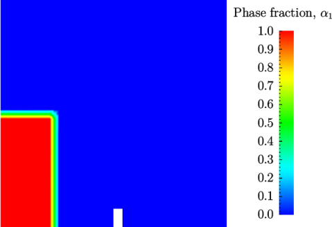
Post-processing of the results can now be done in the usual way. The user can monitor the development of the phase fraction alpha.water in time, e.g. see Figure 2.17 .
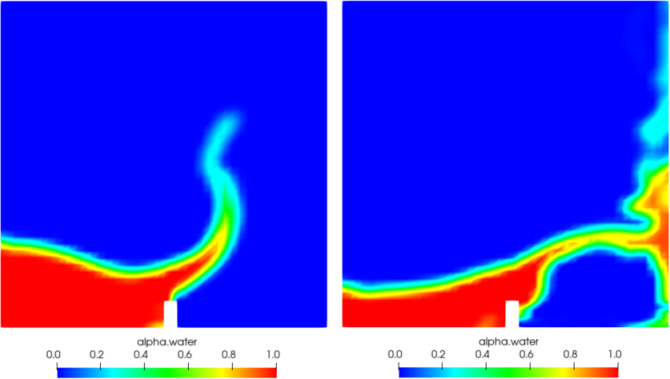
 at
at  = 0.25 s
(left) and 0.50 s (right).
= 0.25 s
(left) and 0.50 s (right).2.2.13 Running in parallel
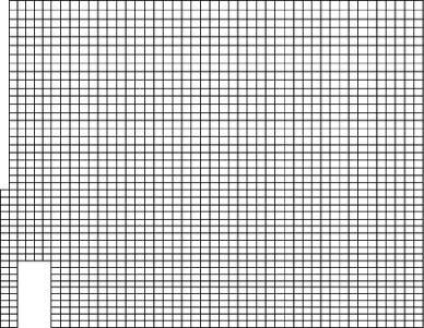
The results from the previous example are generated using a fairly coarse mesh. We now wish to increase the mesh resolution and re-run the case. Using a finer mesh, we can then demonstrate the parallel processing capability of OpenFOAM.
The user should first clone the damBreakLaminar case, e.g. by
run
foamCloneCase damBreakLaminar damBreakLaminarFine
blocks
(
hex (0 1 5 4 12 13 17 16) (46 10 1) simpleGrading (1 1 1)
hex (2 3 7 6 14 15 19 18) (40 10 1) simpleGrading (1 1 1)
hex (4 5 9 8 16 17 21 20) (46 76 1) simpleGrading (1 2 1)
hex (5 6 10 9 17 18 22 21) (4 76 1) simpleGrading (1 2 1)
hex (6 7 11 10 18 19 23 22) (40 76 1) simpleGrading (1 2 1)
);
As the mesh has now changed from the damBreakLaminar example, the user must re-initialise the phase field alpha.water in the 0 time directory since it contains a number of elements that is inconsistent with the new mesh. Note that there is no need to change the U and p_rgh fields since they are specified as uniform which is independent of the number of elements in the field.
The user should then rerun the setFields utility. However, the mesh size is now inconsistent with the number of elements in the alpha.water file in the 0 directory, so the user must delete that file so that setFields uses the original alpha.water.orig file.
rm 0/alpha.water
setFields
Parallel computing uses domain decomposition, in which the geometry and associated fields are broken into pieces and allocated to separate processors for solution. The first step required to run a parallel case is therefore to decompose the domain using the decomposePar utility. There is a dictionary associated with decomposePar named decomposeParDict which is located in the system directory. Also, sample dictionaries can be found within the etc directory in the OpenFOAM installation, which can be copied to the case directory by running the foamGet script, e.g. (you do not need to do this):
foamGet decomposeParDict
The first entry is numberOfSubdomains which specifies the number of subdomains into which the case will be decomposed, usually corresponding to the number of processors available for the case.
This example uses the simple method of decomposition. It requires
the simpleCoeffs to be
configured according to the following criteria. The domain is split
into pieces, or subdomains, in the  ,
,  and
and  directions, the
number of subdomains in each direction being given by the vector
directions, the
number of subdomains in each direction being given by the vector
 . As
this geometry is 2 dimensional, the 3rd direction,
. As
this geometry is 2 dimensional, the 3rd direction,  , cannot be split,
hence
, cannot be split,
hence  must equal 1. The
  and
and  components of split the domain in the
 and
and
 directions and must be specified so that the number of subdomains
specified by
directions and must be specified so that the number of subdomains
specified by  and
and  equals the specified numberOfSubdomains, i.e.
  numberOfSubdomains.
It is beneficial to keep the number of cell faces
adjoining the subdomains to a minimum so, for a square geometry, it
is best to keep the split between the  and directions should
be fairly even. For example, let us assume we wish to run on 4
processors. We would set numberOfSubdomains to 4 and n to (2, 2,
1). The user should run decomposePar by the following command.
and directions should
be fairly even. For example, let us assume we wish to run on 4
processors. We would set numberOfSubdomains to 4 and n to (2, 2,
1). The user should run decomposePar by the following command.
decomposePar
This example presents running in parallel with the openMPI implementation of the standard message-passing interface (MPI). The following command runs on 4 cores of a local multi-processor CPU.
mpirun -np 4 foamRun -parallel
2.2.14 Post-processing a case run in parallel
When the case runs in parallel, the results are written into time directories within the processor<N> sub-directories. The user can confirm this by listing the time directories for the processor0 directory.
ls processor0
It is possible to post-process an individual sub-domain by treating the individual processor directory as a case in its own right. For example, to view the processor1 sub-domain in ParaView, the user can launch paraFoam by running the following command.
paraFoam -case processor1
Alternatively, the decomposed fields and mesh can be reassembled for post-processing in serial. The reconstructPar utility takes the field files from time directories for the processor sub-domain and builds equivalent field files for the complete domain. The user should run the utility as follows.
reconstructPar
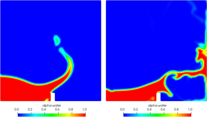
 at
at  = 0.25 s
(left) and 0.50 s (right).
= 0.25 s
(left) and 0.50 s (right).