[version 14][version 13][version 12][version 11][version 10][version 9][version 8][version 7][version 6]
8.3 Transport/rheology models
The momentumTransport file includes any model for the viscous stress in a fluid. That includes turbulence models, described in the previous section 8.2 , but also non-Newtonian and visco-elastic models described in this section. These models are described as laminar, located in $FOAM_SRC/MomentumTransportModels/momentumTransportModels/laminar, including:
- a family of generalisedNewtonian models for a non-uniform
viscosity which is a function of strain rate
 , described in
sections 8.3.1
, 8.3.2,
8.3.3
, 8.3.4
, 8.3.5 and
8.3.6
;
, described in
sections 8.3.1
, 8.3.2,
8.3.3
, 8.3.4
, 8.3.5 and
8.3.6
; - a set of visco-elastic models, including Maxwell, Giesekus and PTT (Phan-Thien & Tanner), described in sections 8.3.7 , 8.3.8 and 8.3.9 , respectively;
- the lambdaThixotropic model, described in section 8.3.10 .
When turbulence modelling is selected in the momentumTransport file, the generalisedNewtonian model is used by default to calculate the molecular viscosity. The choice of generalisedNewtonian model, specified by the viscosityModel keyword, is set to Newtonian by default, which simply uses the viscosity nu specified in the physicalProperties file. The following example exposes the default settings used with turbulence modelling.
simulationType RAS
RAS
{
model kEpsilon; // RAS model
turbulence on;
printCoeffs on;
// "laminar" model generalisedNewtonian is used by default
viscosityModel Newtonian; // default
}
When turbulence modelling is not selected, by setting the laminar simulation type, the user can select any of the laminar models through the model keyword entry in the laminar sub-dictionary, including the visco-elastic models. The laminar models are listed by the following command.
foamToC -table laminarincompressibleMomentumTransportModel
foamToC -table generalisedNewtonianViscosityModel
simulationType laminar
laminar
{
model generalisedNewtonian;
viscosityModel BirdCarreau;
// ... followed by the BirdCarreau parameters
}
 (nu) specified in the physicalProperties file, e.g.
viscosityModel constant;
nu 1.5e-05;
 as the zero strain-rate viscosity
 .
The visco-elastic models incorporate a linear viscous stress using
, in
addition to stress calculated by the respective models. The details
of the models are provided in the following sections.
.
The visco-elastic models incorporate a linear viscous stress using
, in
addition to stress calculated by the respective models. The details
of the models are provided in the following sections.
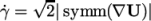
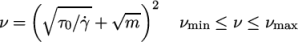
8.3.1 Bird-Carreau model
The Bird-Carreau generalisedNewtonian model is
![a(n−1)∕a ν = ν∞ + (ν0 − ν∞)[1 + (k ˙γ) ] \relax \special {t4ht=](img/index528x.png) |
(8.22) |
 has a default value of 2. An example
specification of the model in momentumTransport is:
has a default value of 2. An example
specification of the model in momentumTransport is:
viscosityModel BirdCarreau;
nuInf 1e-05;
k 1;
n 0.5;
 , is specified by
nu in the physicalProperties file.
, is specified by
nu in the physicalProperties file.
8.3.2 Cross Power Law model
The Cross Power Law generalisedNewtonian model is:
 |
(8.23) |
viscosityModel CrossPowerLaw;
nuInf 1e-05;
m 1;
n 0.5;
 , is specified by
nu in the physicalProperties file.
, is specified by
nu in the physicalProperties file.
8.3.3 Power Law model
The Power Law
generalisedNewtonian model provides a
function for viscosity, limited by minimum and maximum values,
 and
and
 respectively. The function is:
 |
(8.24) |
viscosityModel powerLaw;
nuMax 1e-03;
nuMin 1e-05;
k 1e-05;
n 0.5;
8.3.4 Herschel-Bulkley model
The
Herschel-Bulkley generalisedNewtonian model combines the
effects of Bingham plastic and power-law behaviour in a fluid. For
low strain rates, the material is modelled as a very viscous fluid
with viscosity  . Beyond a threshold in strain-rate corresponding to
threshold stress
. Beyond a threshold in strain-rate corresponding to
threshold stress  , the viscosity is described by a power law. The model
is:
, the viscosity is described by a power law. The model
is:
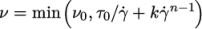 |
(8.25) |
viscosityModel HerschelBulkley;
tau0 0.01;
k 0.001;
n 0.5;
 , is specified in
the physicalProperties file.
, is specified in
the physicalProperties file.
8.3.5 Casson model
The Casson generalisedNewtonian model is a basic model
used in blood rheology that specifies minimum and maximum
viscosities,  and
and  respectively. Beyond a threshold in strain-rate
corresponding to threshold stress
respectively. Beyond a threshold in strain-rate
corresponding to threshold stress  , the viscosity is
described by a “square-root” relationship. The model is:
, the viscosity is
described by a “square-root” relationship. The model is:
 |
(8.26) |
viscosityModel Casson;
m 3.934986e-6;
tau0 2.9032e-6;
nuMax 13.3333e-6;
nuMin 3.9047e-6;
8.3.6 General strain-rate function
A strainRateFunction generalisedNewtonian model exists that allows a user to specify viscosity as a function of strain rate at run-time. It uses the same Function1 functionality to specify the function of strain-rate, used by time varying properties in boundary conditions described in section 6.4.4 . An example specification of the model in momentumTransport is shown below using the polynomial function:
viscosityModel strainRateFunction;
function polynomial ((0 0.1) (1 1.3));
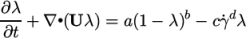
8.3.7 Maxwell model
The Maxwell laminar visco-elastic model solves an
equation for the fluid stress tensor  :
:
![∂τ- ∙ ∙ νM- 1- ∂t + ∇ (U τ) = 2 symm [τ ∇U ]− 2 λ symm (∇U )− λ τ \relax \special {t4ht=](img/index545x.png) |
(8.27) |
 (nuM) is the “Maxwell”
viscosity and
(nuM) is the “Maxwell”
viscosity and  (lambda) is the
relaxation time. An example specification of model parameters is
shown below:
(lambda) is the
relaxation time. An example specification of model parameters is
shown below:
simulationType laminar;
laminar
{
model Maxwell;
MaxwellCoeffs
{
nuM 0.002;
lambda 0.03;
}
}
 , is
specified in the physicalProperties file, the model becomes
equivalent to an Oldroyd-B visco-elastic model. The Maxwell model
includes a multi-mode option where
, is
specified in the physicalProperties file, the model becomes
equivalent to an Oldroyd-B visco-elastic model. The Maxwell model
includes a multi-mode option where  is a sum of stresses,
each with an associated relaxation time
is a sum of stresses,
each with an associated relaxation time  .
.
8.3.8 Giesekus model
The Giesekus laminar visco-elastic model is similar to
the Maxwell model but includes an additional “mobility” term in the
equation for :
![∂-τ ∙ ∙ νM- 1- αG- ∙ ∂t + ∇ (U τ) = 2symm [τ∇U ]− 2 λ symm (∇U )− λτ − νM [τiτi] \relax \special {t4ht=](img/index552x.png) |
(8.28) |
 (alphaG) is the
mobility parameter. An example specification of model parameters is
shown below:
(alphaG) is the
mobility parameter. An example specification of model parameters is
shown below:
simulationType laminar;
laminar
{
model Giesekus;
GiesekusCoeffs
{
nuM 0.002;
lambda 0.03;
alphaG 0.1;
}
}
 is a sum of
stresses, each with an associated relaxation time
is a sum of
stresses, each with an associated relaxation time  and mobility
coefficient
and mobility
coefficient  .
.
8.3.9 Phan-Thien-Tanner (PTT) model
The
Phan-Thien-Tanner (PTT) laminar
visco-elastic model is also similar to the Maxwell model but
includes an additional “extensibility” term in the equation for
 ,
suitable for polymeric liquids:
,
suitable for polymeric liquids:
![( ) ∂τ- νM- 1- 𝜀λ- ∂t + ∇ ∙(U τ) = 2 symm [τ∙∇U ]− 2 λ symm (∇U ) − λ exp − ν tr(τ) τ M \relax \special {t4ht=](img/index558x.png) |
(8.29) |
 (epsilon) is the
extensibility parameter. An example specification of model
parameters is shown below:
(epsilon) is the
extensibility parameter. An example specification of model
parameters is shown below:
simulationType laminar;
laminar
{
model PTT;
PTTCoeffs
{
nuM 0.002;
lambda 0.03;
epsilon 0.25;
}
}
 is a sum of
stresses, each with an associated relaxation time
is a sum of
stresses, each with an associated relaxation time  and extensibility
coefficient
and extensibility
coefficient  .
.
8.3.10 Lambda thixotropic model
The Lambda
Thixotropic laminar model calculates the
evolution of a structural parameter (lambda) according to:
 |
(8.30) |
 ,
,  ,
,  and
and  . The viscosity
  is then calculated
according to:
is then calculated
according to:
 |
(8.31) |
 . The viscosities
  and
and  are limiting values
corresponding to
are limiting values
corresponding to  and
and  .
.
An example specification of the model in momentumTransport is:
simulationType laminar;
laminar
{
model lambdaThixotropic;
lambdaThixotropicCoeffs
{
a 1;
b 2;
c 1e-3;
d 3;
nu0 0.1;
nuInf 1e-4;
}
}