[version 11][version 10][version 9][version 8][version 7][version 6]
2.1 Backward-facing step
This tutorial will describe how to pre-process, run and post-process a case involving isothermal, incompressible flow across a backward-facing step. The problem is treated as two dimensional with the geometry shown in Figure 2.1. The domain consists of:
- an inlet opening (left);
- an outlet opening (right);
- an upper wall, which is horizontal before tapering gently toward the outlet;
- a lower wall, which also tapers towards the outlet, but includes an abrupt step within a short distance from the inlet;
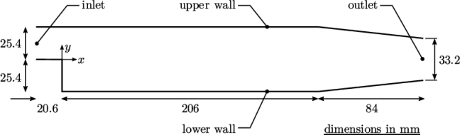
Flow enters the inlet in the  -direction with a speed of
10 m/s. The flow will be assumed isothermal and incompressible
and will be solved using the incompressibleFluid modular
solver.
-direction with a speed of
10 m/s. The flow will be assumed isothermal and incompressible
and will be solved using the incompressibleFluid modular
solver.
2.1.1 Pre-processing
Cases are configured in OpenFOAM by editing input data files. Users should select a suitable file editor to do this, e.g. emacs, vi, gedit, nedit, etc. A case involves multiple data files, corresponding to different parts of the configuration, e.g. mesh, fields, properties, control parameters, etc. As described in section 4.1 , the set of files is stored within a case directory, which is given a suitably descriptive name. This tutorial uses the case $FOAM_TUTORIALS/incompressibleFluid/pitzDailySteady, which the user should copy to their run directory as follows.
cd $FOAM_RUN
cp -r $FOAM_TUTORIALS/modules/incompressibleFluid/pitzDailySteady .
cd pitzDailySteady
2.1.2 Mesh generation
OpenFOAM always operates in a three dimensional Cartesian coordinate system and all geometries are generated in three dimensions (3D). It solves the case in two dimensions (2D) by specifying a special empty boundary condition on boundaries normal to the (3rd) dimension (for which no solution is required).
OpenFOAM includes a simple mesh generator, blockMesh, which generates meshes from a blockMeshDict file, located in the system directory for a given case. The domain is defined using blocks whose vertex locations are specified in the file. The structure of the blocks and respective vertices are shown in Figure 2.2 .
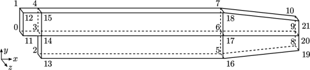
The backwardStep domain consists of five blocks
shown in the figure. The domain depth in the  direction (exaggerated in
the figure) is 1 mm. The blockMeshDict file for this example is
reproduced below:
direction (exaggerated in
the figure) is 1 mm. The blockMeshDict file for this example is
reproduced below:
2 ========= |
3 \\ / F ield | OpenFOAM: The Open Source CFD Toolbox
4 \\ / O peration | Website: https://openfoam.org
5 \\ / A nd | Version: dev
6 \\/ M anipulation |
7\*---------------------------------------------------------------------------*/
8FoamFile
9{
10 format ascii;
11 class dictionary;
12 object blockMeshDict;
13}
14// * * * * * * * * * * * * * * * * * * * * * * * * * * * * * * * * * * * * * //
15
16// Note: this file is a Copy of $FOAM_TUTORIALS/resources/blockMesh/pitzDaily
17
18convertToMeters 0.001;
19
20vertices
21(
22 (-20.6 0 -0.5)
23 (-20.6 25.4 -0.5)
24 (0 -25.4 -0.5)
25 (0 0 -0.5)
26 (0 25.4 -0.5)
27 (206 -25.4 -0.5)
28 (206 0 -0.5)
29 (206 25.4 -0.5)
30 (290 -16.6 -0.5)
31 (290 0 -0.5)
32 (290 16.6 -0.5)
33
34 (-20.6 0 0.5)
35 (-20.6 25.4 0.5)
36 (0 -25.4 0.5)
37 (0 0 0.5)
38 (0 25.4 0.5)
39 (206 -25.4 0.5)
40 (206 0 0.5)
41 (206 25.4 0.5)
42 (290 -16.6 0.5)
43 (290 0 0.5)
44 (290 16.6 0.5)
45);
46
47negY
48(
49 (2 4 1)
50 (1 3 0.3)
51);
52
53posY
54(
55 (1 4 2)
56 (2 3 4)
57 (2 4 0.25)
58);
59
60posYR
61(
62 (2 1 1)
63 (1 1 0.25)
64);
65
66
67blocks
68(
69 hex (0 3 4 1 11 14 15 12)
70 (18 30 1)
71 simpleGrading (0.5 $posY 1)
72
73 hex (2 5 6 3 13 16 17 14)
74 (180 27 1)
75 edgeGrading (4 4 4 4 $negY 1 1 $negY 1 1 1 1)
76
77 hex (3 6 7 4 14 17 18 15)
78 (180 30 1)
79 edgeGrading (4 4 4 4 $posY $posYR $posYR $posY 1 1 1 1)
80
81 hex (5 8 9 6 16 19 20 17)
82 (25 27 1)
83 simpleGrading (2.5 1 1)
84
85 hex (6 9 10 7 17 20 21 18)
86 (25 30 1)
87 simpleGrading (2.5 $posYR 1)
88);
89
90boundary
91(
92 inlet
93 {
94 type patch;
95 faces
96 (
97 (0 1 12 11)
98 );
99 }
100 outlet
101 {
102 type patch;
103 faces
104 (
105 (8 9 20 19)
106 (9 10 21 20)
107 );
108 }
109 upperWall
110 {
111 type wall;
112 faces
113 (
114 (1 4 15 12)
115 (4 7 18 15)
116 (7 10 21 18)
117 );
118 }
119 lowerWall
120 {
121 type wall;
122 faces
123 (
124 (0 3 14 11)
125 (3 2 13 14)
126 (2 5 16 13)
127 (5 8 19 16)
128 );
129 }
130 frontAndBack
131 {
132 type empty;
133 faces
134 (
135 (0 3 4 1)
136 (2 5 6 3)
137 (3 6 7 4)
138 (5 8 9 6)
139 (6 9 10 7)
140 (11 14 15 12)
141 (13 16 17 14)
142 (14 17 18 15)
143 (16 19 20 17)
144 (17 20 21 18)
145 );
146 }
147);
148
149// ************************************************************************* //
The file first contains header information in the form of a banner (lines 1-7), then file information contained in a FoamFile sub-dictionary, delimited by curly braces ({…}).
For the remainder of the manual:
To save space, file headers, including the banner and FoamFile sub-dictionary, will be removed
from further verbatim quoting of case files.
The body of the blockMeshDict file will be briefly reviewed here, but for further details see section 5.4 . The file begins with the coordinates of the block vertices. All vertices are scaled by the factor specified by convertToMeters. The file then defines the blocks (here, 5 of them). Each block is a hexahedral shape, given by the hex entry. The eight vertex labels are listed following the hex entry.
The number of cells is specified in each direction
for each block by a vector of three integers. For example the first
block specifies (18 30 1), which
produces 18 cells through the block in the -direction, 30 in the
 -direction and 1 in the
  -direction (the unused
direction).
-direction (the unused
direction).
The blocks includes mesh grading, which enables the cell lengths to vary across the block. It is includes multi-grading which is described in section 5.4.5 using parameters negY, posY and posYR.
Finally, the mesh splits the boundary into inlet,
outlet and wall regions, included in the following patches:
upperWall and lowerWall for the wall boundaries of the
domain; inlet and outlet for the open boundaries. The
boundary in the -normal direction is included in a single patch named
frontAndBack.
The mesh is generated by running blockMesh on this blockMeshDict file. From within the case directory, this is done, simply by typing in the terminal:
blockMesh
2.1.3 Viewing the mesh
It is sensible to verify the mesh is generated correctly before running the simulation. The mesh can be viewed in ParaView, the post-processing tool supplied with OpenFOAM. The ParaView post-processing is conveniently launched on OpenFOAM case data by executing the paraFoam script from within the case directory.
Any UNIX/Linux executable (application, script, etc.) can be run in two ways: as a foreground process, i.e. one in which the shell waits until the executable has finished before returning the command prompt; or, as a background process, which allows the shell to accept additional commands while the executable is still running. Since it is convenient to keep ParaView open while running other commands from the terminal, we will launch it in the background using the & operator by typing
paraFoam &
This launches the ParaView window as shown in
Figure 7.1
. In the Pipeline Browser, ParaView registers pitzDailySteady.OpenFOAM, representing the
pitzDailySteady case.
For the
remainder of the manual:
The first time ParaView is
launched, users are faced with a splash screen which can be
permanently deactivated by clicking the relevant checkbox before
closing.
Before clicking the Apply button, the user can select some geometry from the Mesh Parts panel in the Properties window (may require scrolling to find). Because the case is small, it is easiest to select all the data by checking the box adjacent to the Mesh Parts panel title, which automatically checks all individual components within the respective panel. The user should then click the Apply button to load the geometry into ParaView.
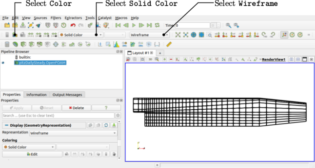
The user can control the visual representation of the selected module either using the second row of controls at the top of ParaView or by scrolling down further to the Display panel that. The user should make the selections using the second row of controls as shown in Figure 2.3 , or as described below from within the Display panel.
- in the Coloring section, select Solid Color;
- click Edit (in Coloring) and select an appropriate colour e.g. black (for a white background);
- select Wireframe from the Representation menu.
Especially the first time the user starts ParaView, it is recommended that they manipulate the view as described in section 7.1.5 . In particular, since this is a 2D case, it is recommended that Camera Parallel Projection is selected at the bottom of the View (Render View) panel. The selection can be saved as a user default by clicking the Save current view settings button to the right of the View (Render View) heading (the furthest right of the four buttons). The background colour can be also set in the View (Render View) panel at the bottom of the Properties window.
Note that, many
parameters in the Properties window are only visible by clicking the Advanced Properties gearwheel button (  ) at the top of
the Properties window, next to
the search box.
) at the top of
the Properties window, next to
the search box.
2.1.4 Boundary and initial conditions
Once the mesh generation is complete, the user
can look at the configuration of the initial fields for this case.
The case starts at time  s, so the initial field data is stored in a
0 sub-directory of the
cavity directory. The
0 sub-directory contains
several files including p and
U, which represent the
pressure (
s, so the initial field data is stored in a
0 sub-directory of the
cavity directory. The
0 sub-directory contains
several files including p and
U, which represent the
pressure ( ) and velocity (
 ) fields, respectfully. Within these files the
initial values and boundary conditions must be set. Let us examine
the p file below.
) fields, respectfully. Within these files the
initial values and boundary conditions must be set. Let us examine
the p file below.
17
18internalField uniform 0;
19
20boundaryField
21{
22 inlet
23 {
24 type zeroGradient;
25 }
26
27 outlet
28 {
29 type fixedValue;
30 value uniform 0;
31 }
32
33 upperWall
34 {
35 type zeroGradient;
36 }
37
38 lowerWall
39 {
40 type zeroGradient;
41 }
42
43 frontAndBack
44 {
45 type empty;
46 }
47}
48
49// ************************************************************************* //
There are three principal entries in field data files:
- dimensions
- specifies the dimensions of the field, here
kinematic pressure,
i.e.
 (see
section 4.2.6
for more
information);
(see
section 4.2.6
for more
information); - internalField
- the internal field data which can be uniform, described by a single value; or nonuniform, where the values of the field must be specified for all cells (see section 4.2.8 for more information);
- boundaryField
- the boundary field data that includes boundary conditions and data for all the boundary patches (see section 4.2.8 for more information).
For this pitzDailySteady case, the initial fields are set to be uniform. Here the pressure is kinematic, and since the solution does not involve energy and thermodynamics, its absolute value is not relevant, so is set to uniform 0 for convenience.
The boundary includes the upperWall, lowerWall, inlet and outlet patches. The walls and inlet are both assigned the zeroGradient boundary condition for p, meaning “the normal gradient of pressure is zero”. The outlet uses the fixedValue boundary condition for p with value of uniform 0. The frontAndBack patch, describing the front and back planes of the 2D case, is specified as empty.
The user can similarly examine the velocity field in the 0/U file. The dimensions are those expected for velocity, the internal field is initialised as uniform zero, which in the case of velocity must be expressed by 3 vector components, i.e. uniform (0 0 0) (see section 4.2.5 for more information).
A no-slip condition is assumed on the walls,
specified by a noSlip condition. The inlet flow speed
is 10 m/s in the  -direction so represented by a fixedValue condition with value of uniform (10 0 0). The outlet reverts to the
zeroGradient condition. The
frontAndBack patch must be set
to empty.
-direction so represented by a fixedValue condition with value of uniform (10 0 0). The outlet reverts to the
zeroGradient condition. The
frontAndBack patch must be set
to empty.
2.1.5 Physical properties
Physical properties and model configurations for the case are stored in dictionary files in the constant directory. Properties for this example are specified in the following physicalProperties file.
17viscosityModel constant;
18
19nu 1e-05;
20
21// ************************************************************************* //
First it includes the viscosityModel entry which is set to constant. With that model, a single
kinematic viscosity is then specified by the keyword nu, representing the Greek symbol  phonetically for the
kinematic viscosity. The value is set to
phonetically for the
kinematic viscosity. The value is set to 
 .
.
2.1.6 Momentum transport
An estimate of the Reynolds number is required to determine whether the flow is expected to be turbulent. The Reynolds number is defined as:
 |
(2.1) |
 and
and  are the characteristic speed and length respectively and
 is
the kinematic viscosity. Using the inlet (or
step) height
is
the kinematic viscosity. Using the inlet (or
step) height  25.4 mm and
  10 m/s,
 25400. For flow in a pipe, transition typically occurs
when
25400. For flow in a pipe, transition typically occurs
when  2000, so this case can be assumed to be turbulent.
The momentumTransport file characterises the viscous stress in the fluid by a variety of models, e.g. Newtonian and non-Newtonian fluids, turbulence, visco-elasticity and more. For this example, the file includes the configuration of turbulence modelling as shown below.
17simulationType RAS;
18
19RAS
20{
21 // Tested with kEpsilon, realizableKE, kOmega, kOmega2006, kOmegaSST, v2f,
22 // ShihQuadraticKE, LienCubicKE.
23 model kEpsilon;
24
25 turbulence on;
26
27 printCoeffs on;
28
29 viscosityModel Newtonian;
30}
31
32
33// ************************************************************************* //
The type of simulation is first specified by the
simulationType keyword. The RAS entry indicates a Reynolds-averaged simulation,
the standard form of turbulence modelling. The RAS sub-dictionary includes the
model entry which is set to the
well-known  –
– model by the kEpsilon entry. The turbulence keyword provides a switch to turn the modelling on
and off. The model coefficients have default values which can be
overridden with additional entries in the momentumTransport file. When the
printCoeffs switch in on, the
coefficients are printed to the terminal when the case is run. The
viscosityModel entry confirms
the fluid is modelled as Newtonian (which is the default model, so
the entry could be omitted).
model by the kEpsilon entry. The turbulence keyword provides a switch to turn the modelling on
and off. The model coefficients have default values which can be
overridden with additional entries in the momentumTransport file. When the
printCoeffs switch in on, the
coefficients are printed to the terminal when the case is run. The
viscosityModel entry confirms
the fluid is modelled as Newtonian (which is the default model, so
the entry could be omitted).
The  –
– model solves transport equations for:
, the
turbulent kinetic energy; and, , the turbulent
dissipation rate. The initial and boundary
conditions for those fields are configured in the 0/k and 0/epsilon files, respectfully.
model solves transport equations for:
, the
turbulent kinetic energy; and, , the turbulent
dissipation rate. The initial and boundary
conditions for those fields are configured in the 0/k and 0/epsilon files, respectfully.
In particular, the turbulent fields must be
initialised with suitable internal and inlet values. Turbulent
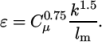
kinetic energy  can be calculated by
 |
(2.2) |
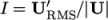 , the ratio of the
root-mean-square (RMS) of turbulent fluctuations
, the ratio of the
root-mean-square (RMS) of turbulent fluctuations  to the mean flow
speed
to the mean flow
speed  . This example uses an estimate
  , such that
  In the
0/k file, 0.375 is used both for the initial
internalField and the inlet
value.
In the
0/k file, 0.375 is used both for the initial
internalField and the inlet
value.
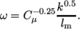
The turbulent dissipation rate  can be calculated
by
can be calculated
by
 |
(2.3) |
 and an estimate of Prandtl mixing length
  . This example uses an
estimate
. This example uses an
estimate  step height = 2.54 mm, such that
  In the 0/epsilon file, 14.855 is used both for the initial
internalField and the inlet
value.
In the 0/epsilon file, 14.855 is used both for the initial
internalField and the inlet
value.
The turbulence model is deployed with wall
functions to model the behaviour at wall boundaries. Wall functions
are applied as boundary conditions on the individual wall patches
which enables different wall function models to be applied to
different wall regions. The choice of wall function models are
specified through the turbulent viscosity field,  in the 0/nut file.
17dimensions [0 2 -1 0 0 0 0];
18
19internalField uniform 0;
20
21boundaryField
22{
23 inlet
24 {
25 type calculated;
26 value uniform 0;
27 }
28 outlet
29 {
30 type calculated;
31 value uniform 0;
32 }
33 upperWall
34 {
35 type nutkWallFunction;
36 value uniform 0;
37 }
38 lowerWall
39 {
40 type nutkWallFunction;
41 value uniform 0;
42 }
43 frontAndBack
44 {
45 type empty;
46 }
47}
48
49
50// ************************************************************************* //
This case uses standard wall functions, specified by the nutkWallFunction type on the upperWall and lowerWall patches. Alternative wall function models include the rough wall functions, specified through the nutRoughWallFunction keyword.
When wall functions are specified through boundary
conditions in the 0/nut file,
corresponding conditions must be applied to the wall patches for
the turbulence fields. The 0/eps and 0/k files show that  is assigned the
epsilonWallFunction condition
and
is assigned the
epsilonWallFunction condition
and  is assigned the kqRWallFunction
condition at the wall patches. The latter is a generic boundary
condition that can be applied to any field that are of a turbulent
kinetic energy type, e.g.
is assigned the kqRWallFunction
condition at the wall patches. The latter is a generic boundary
condition that can be applied to any field that are of a turbulent
kinetic energy type, e.g.  ,
,  or Reynolds Stress
 .
.
2.1.7 Control
Input data relating to the control of time and reading and writing of the solution data are read in from the controlDict file. The user should view this file; as a case control file, it is located in the system directory.
17application foamRun;
18
19solver incompressibleFluid;
20
21startFrom startTime;
22
23startTime 0;
24
25stopAt endTime;
26
27endTime 2000;
28
29deltaT 1;
30
31writeControl timeStep;
32
33writeInterval 100;
34
35purgeWrite 0;
36
37writeFormat ascii;
38
39writePrecision 6;
40
41writeCompression off;
42
43timeFormat general;
44
45timePrecision 6;
46
47runTimeModifiable true;
48
49cacheTemporaryObjects
50(
51 kEpsilon:G
52);
53
54functions
55{
56 #includeFunc streamlinesLine
57 (
58 name=streamlines,
59 start=(-0.0205 0.001 0.00001),
60 end=(-0.0205 0.0251 0.00001),
61 nPoints=10,
62 fields=(p k U)
63 )
64
65 #includeFunc writeObjects(kEpsilon:G)
66}
67
68// ************************************************************************* //
The file first includes an application entry which is not used by OpenFOAM. It is instead used by run scripts, named Allrun, which are accompany many of the example cases. The following solver entry describes the solver module used for the simulation. This example uses the incompressibleFluid module for steady or transient turbulent flow of incompressible isothermal fluids with optional mesh motion and change.
The start/stop times and the time step for the
run must be set. OpenFOAM provides flexible options for time
controls which are described in section 4.4
. Like most cases, this
example starts the simulation at time  which instructs the
solver to read its field data from a directory named 0. Therefore we set the startFrom keyword to startTime and then specify the startTime keyword to be 0.
which instructs the
solver to read its field data from a directory named 0. Therefore we set the startFrom keyword to startTime and then specify the startTime keyword to be 0.
The aim of the simulation is to reach the steady
solution where the recirculation region is fully developed adjacent
to the step. The incompressibleFluid module can run as a
steady-state solver by setting the time derivatives  to zero in all the
equations. This is achieved by setting the ddtSchemes to steadyState in the fvSchemes file, discussed later.
to zero in all the
equations. This is achieved by setting the ddtSchemes to steadyState in the fvSchemes file, discussed later.
In this mode, the time step, represented by the
keyword deltaT, is only used as
a time increment (since it is no longer used to discretise
).
Its value does not affect the solution, so for steady solutions it
is set to 1 so that time simply
represents the number of solution steps.
The endTime keyword sets a time at which the solver application stops running. The value of 2000 provides an adequate number of solution steps to enable the steady solution to converge to a reasonable level of accuracy.
As the simulation progresses we wish to write
results at intervals of time of interest for visualisation and
other post-processing. The writeControl keyword presents several options for setting the
time at which the results are written; here the timeStep option specifies that results are written every
 th
time step where the value is specified under the writeInterval keyword. The interval of 100 means results are written at 100, 200,
etc.
th
time step where the value is specified under the writeInterval keyword. The interval of 100 means results are written at 100, 200,
etc.
OpenFOAM creates a new directory named after the current time, e.g. 100, on each occasion that it writes a set of data, as discussed in full in section 4.1 . It writes out the results for each solution field, e.g. U, p, k, into the time directories.
2.1.8 Discretisation and linear-solver settings
The user specifies the choice of finite volume discretisation schemes in the fvSchemes file in the system directory. The specification of the linear equation solvers and tolerances and other algorithm controls is made in the fvSolution file, also in the system directory.
The details of those two files are described in Sections 4.5 and 4.6 , respectively. For this example, the following points are important:
- the ddtSchemes defaults to steadyState in fvSchemes, to invoke a steady-state calculation;
- steady-state solution uses an algorithm based on SIMPLE whose controls are configured in a SIMPLE sub-dictionary in the fvSolution file;
- the SIMPLE sub-dictionary contains the consistent switch which is set to yes, applying the “consistent” form of the SIMPLE algorithm (SIMPLEC);
- the convergence of SIMPLEC is very sensitive to the relaxationFactors in the fvSolution file; the values of 0.9 are carefully tuned and are not suitable for the standard SIMPLE algorithm;
- SIMPLEC’s sensitive convergence generally makes it only reliable for cases with simple geometries.
2.1.9 Running an application
To run a simulation with a single domain region, the foamRun application is run. It loads the relevant solver module, from the solver entry in the controlDict file, to perform the calculation. On this occasion, we will run foamRun in the terminal foreground by typing the following from within the case directory.
foamRun
The progress of the simulation is reported in the terminal window. It describes successive solutions steps, giving the initial and final residuals for each equation, and conservation errors.
The SIMPLE algorithm controls in fvSolution include a residualControl sub-dictionary with a set of tolerances for p, U and turbulence fields. The incompressibleFluid solver terminates When the initial residuals for all fields fall below their respective tolerances. In this example, the solver terminates at 287 iterations with the following statement.
SIMPLE solution converged in 287 iterations
2.1.10 Time selection in ParaView
Once the results are written to time directories, they can be viewed using ParaView. The first step is to activate the time selector, including the Time text box on right hand side of the top row of buttons, as shown in Figure 7.4 .
If ParaView is opened before there are any solution time directories (i.e. only a 0 directory), the time selector must later be re-activated to recognise the solution time directories by:
- selecting the top of the Properties window (scroll up the panel if necessary) in ParaView;
- toggling the Cache Mesh button at the top of the panel (under the Refresh Times button;
- clicking the Apply button.
The time selector is then updated with Time becoming a drop down menu with the time directories from the case (0, 100, 200 and 287). In order to view the solution at 287, the user can use the VCR Controls or Current Time Controls to change the current time to 287.
For the remainder of the manual:
In ParaView, if the window
panels, e.g. Properties, do not contain the expected
entries, ensure that the relevant module is highlighted in blue in
the Pipeline Browser. For
example, Refresh Times only
appears when the top module (here, pitzDailySteady.OpenFOAM) is
selected.
2.1.11 Colouring surfaces
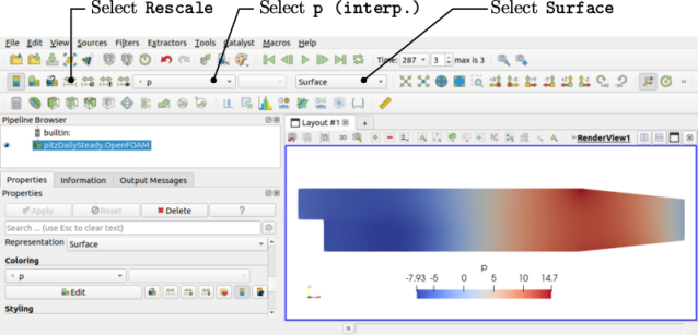
To view pressure, the user can either make selections from the second row of buttons at the top of ParaView as shown in Figure 2.4 or scroll down to the Display panel in Properties and make the following selections:
- select Surface from the Representation menu;
- select
 in
Coloring
in
Coloring - click the Rescale button to set the colour scale to the data range, if necessary.
The pressure field should appear as shown above,
with the pressure increasing to a maximum at the contraction of the
channel towards the outlet. With the point icon ( ), the
pressure field is interpolated across each cell to give a continuous
appearance. Instead if the user selects the cell icon, (
 ), from the Coloring menu, a single value for pressure
will be attributed to each cell, represented by a single colour
with no grading.
), from the Coloring menu, a single value for pressure
will be attributed to each cell, represented by a single colour
with no grading.
A colour legend is included which can be disabled by clicking the Toggle Color Legend Visibility button at the left of the second row of buttons at the top of ParaView. These buttons are part of the Active Variable Controls toolbar, shown in Figure 7.4 ). The Edit Color Map button, second on the left in Active Variable Controls toolbar, opens the Color Map Editor window, as shown in Figure 2.5 , where the user can set a range of attributes of the colour scale and the color bar.
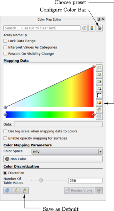
In particular, ParaView defaults to using a colour scale of blue to white to red rather than the more common blue to green to red (rainbow). Therefore the first time that the user executes ParaView, they may wish to change the colour scale. This can be done by selecting the Choose Preset button (with the heart icon) in the Color Scale Editor. The conventional color scale for CFD is Blue to Red Rainbow which is only listed if the user types the name in the Search bar or checks the gearwheel to the right of that bar.
After selecting Blue to Red Rainbow and clicking Apply and Close, the user can click the Save as Default button at the absolute bottom of the panel (file save symbol) so that ParaView will always adopt this type of colour bar.
The user can also edit the color legend properties, such as text size, font selection and numbering format for the scale, by clicking the Edit Color Legend Properties to the far right of the search bar, as shown in Figure 2.5 .
2.1.12 Cutting plane (slice)
If the user rotates the image, by holding down the left mouse button in the image window and moving the cursor, they can see that they have now coloured the complete geometry surface by the pressure. In order to produce a 2D contour plot the user should first create a cutting plane, or ‘slice’. With the pitzDailySteady.OpenFOAM module highlighted in the Pipeline Browser, the user should select the Slice filter from the Filters menu in the top menu of ParaView (accessible at the top of the screen on some systems). The Slice filter can be found in the Common sub-menu or among the Common and Data Analysis buttons, the third row of buttons at the top of ParaView (see Figure 7.4 ).
Selecting the Slice filter creates a new item in the
Pipeline Browser. In the
Properties window, the cutting
plane should have an origin at a point on the  -axis, e.g.
  and its normal should be set to
 (click the Z Normal button).
When Apply is
clicked, the slice appears in the RenderView window, while the original
pitzDailySteady.OpenFOAM module
disappears. The visibility of each module is enabled and disabled
by the eye button to the left
of each module in the pipeline browser. For the remainder of
the manual:
In ParaView, if items do not
appear to be displayed in the RenderView window, ensure the relevant
module is visible by switching on the eye button in the Pipeline Browser.
2.1.13 Vector plots
Before drawing vectors of the flow velocity, turn off the display of the Slice module by highlighting it in the Pipeline Browser and clicking the eye button to the left of it. The aim is to generate a vector glyph for velocity at the centre of each cell. We therefore first need to filter the cell centres from the mesh geometry as described in section 7.1.7 . With the pitzDailySteady.OpenFOAM module highlighted in the Pipeline Browser, the user should select Cell Centers from the Filters->Alphabetical menu and then click Apply.
With the Centers highlighted in the Pipeline Browser, the user should then select Glyph from the Filters->Common menu (or the third row of buttons). The Properties window panel should appear as shown in Figure 2.6 .
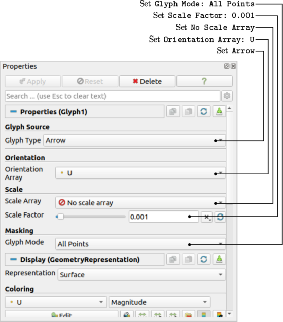
When displaying velocity vectors, there are four principal settings required for the glyphs:
- the glyph type, set to Arrow;
- the arrow direction, set by Orientation Array;
- the arrow lengths, set by Scale Array and Scale Factor;
- the number of arrows, set by Glyph Mode.
On clicking Apply, the glyphs appear as a single colour, e.g. white. The user should colour the glyphs by velocity magnitude which, as usual, is controlled by setting U in the drop down menu towards the left of the second row of buttons.
The Legend is also displayed. The user can configure the legend by clicking Edit Color Map (second button from left, second row). This opens the the Color Map Editor window. The legend can be configured by clicking by the button furthest to the right of the search box. This button opens the Edit Color Legend Properties window. The Advanced Properties gearwheel button should be checked to the right of the search box.
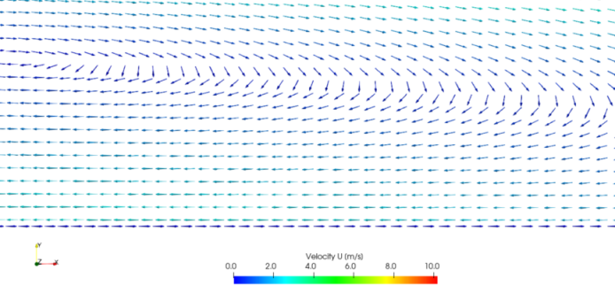
Titles and labels can be fully configured. For Figure 2.7 , the legend title is set to Velocity U [m/s]. The labels are specified to 1 fixed decimal place by unchecking Automatic Label Format and entering %-#6.1f in the Label Format text box. Add Range Labels is also unchecked.
Sample output is shown in Figure 2.7
, zooming in
on part of the recirculation region downstream of the step. At the
lower wall, glyphs point in a direction opposing that of the flow
adjacent to the wall. This glitch is caused by these glyphs being
drawn at the face centres of the wall boundary patch, where the the
velocity magnitude is 0 due to the no-slip condition. Without any
direction to the vectors, ParaView orientates the arrows in a
default  -direction. A quick way to remove these vectors is:
- go back to the pitzDailySteady.OpenFOAM module at the top of the Pipeline Browser;
- in the Mesh Parts panel, uncheck the lowerWall patch;
- click Apply.
2.1.14 Popular filters in ParaView
ParaView includes over 200 filters which can be listed by the Filters->Alphabetical menu. Only a small fraction, e.g. 10-15, of these filters are relevant for CFD, which we suggest adding to the Filters->Favourites menu. To do this, select Manage Favourites from the Filters->Favourites menu. Search for the following important filters and click Add>> to add them to the Favourites menu:
- Extract Block, to select components of the domain, e.g. boundary patches and internal cells;
- Slice, to insert a plane through the geometry;
- Cell Centers and Glyph, principally to draw velocity vectors;
- Stream Tracer and Tube, to draw streamlines;
- Contour, to draw contour lines (on surfaces) and iso-surfaces;
- Feature Edges, to capture features on a surface for better image definition.
2.1.15 Contours
Before drawing contour lines of the flow speed, turn off the display of the Glyph module by highlighting it in the Pipeline Browser and clicking the eye button to its left. The user should then highlight the Slice module and colour by velocity U. We will then aim to draw contour lines on the slice at intervals of U of 1, 2, …, 10.
The contour lines can be drawn by applying the Contour filter to the slice. The filter draws lines in 2D, or surfaces in 3D, along constant values of scalar quantities. Contours cannot be drawn directly from U, since it is a vector, so we first need to generate a scalar field of the magnitude of U.
The mag(U) field can be generated using post-processing with function objects, described in section 7.3 . The user should run the foamPostProcess utility, calling the mag function object using the -func option as follows:
foamPostProcess -func "mag(U)"
The utility loops over all time directories. For each time directory, it reads in U, calculates mag(U) and writes it out as a field file back into the time directory. The mag(U) field must then be loaded into ParaView by: first, from the pitzDailySteady.OpenFOAM in the Pipeline Browser, clicking Refresh Times; then, scrolling down to the Fields panel, selecting mag(U) and clicking Apply.
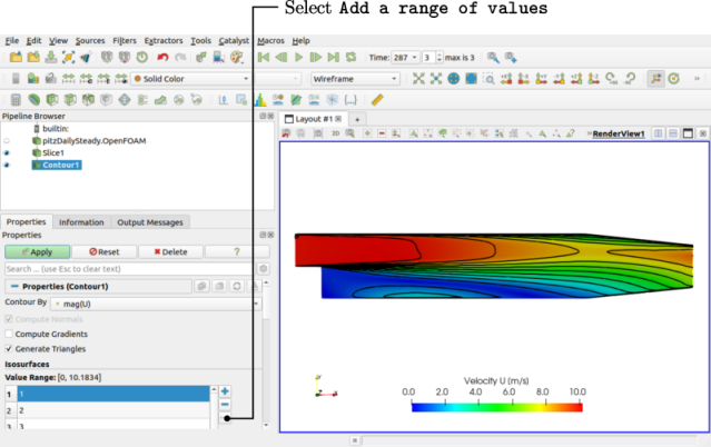
The user should re-select the Slice module in the Pipeline Browser, then apply the Contour filter. In the Properties panel, the user should select mag(U) from the Contour By menu. Under Isosurfaces, the user should first delete the default value by clicking the – button, then add a range of 10 values as shown in Figure 2.8 . The contours can be displayed with a Wireframe representation with solid black Coloring.
2.1.16 Streamline plots
Before drawing streamlines, the user should turn off the display of the Contour module. To display streamlines for this 2D example, the user should first highlight the Slice module in the Pipeline Browser and then apply the Stream Tracer filter.
A new StreamTracer module opens which is
configured through its Properties window. Tracer is created by
tracking lines in the direction of flow, starting from seed points. With Integration Direction BOTH, lines are
tracked both upstream and downstream of the seed points. The user
should scroll down the Properties window to configure the
Seeds. The default Seed Type in Line which seeds points along a line drawn
between specified points. In the Line
Parameters, the user should can set the two points to
 to
to
 . The
Resolution specifies the number
of seed points distributed along the line, which should be reduced
to 25.
. The
Resolution specifies the number
of seed points distributed along the line, which should be reduced
to 25.
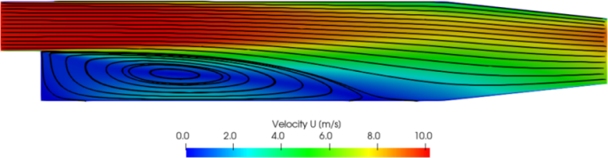
On clicking Apply the tracer is generated as shown in Figure 2.9 . The user can experiment with the line points and resolution to produce different stream tracer output.
2.1.17 Inlet boundary condition
The user should examine the flow at the inlet boundary of the domain. The velocity condition is specified in 0/U as fixedValue with a value of (10 0 0). This value is applied to all faces of the inlet boundary patch. The inlet is adjacent to wall boundaries where the noSlip condition is applied, giving rise to a sudden change in U, between adjacent boundary faces.
The user should zoom in around the inlet region
of the geometry using the right button of the mouse. The
Slice module should be
activated in the Pipeline
Browser and coloured by
cell values of p (  selection). In order to highlight
the variation in pressure in cells close to the inlet, the user
should apply a custom range of
selection). In order to highlight
the variation in pressure in cells close to the inlet, the user
should apply a custom range of  as shown in
Figure 2.10
. A
custom range is applied by clicking the Rescale to Custom Data Range button (
as shown in
Figure 2.10
. A
custom range is applied by clicking the Rescale to Custom Data Range button (
 ), located fifth from the left of the
second row of buttons. A panel opens, in which the minimum and
maximum values of the range should be entered before clicking the
Rescale button.
), located fifth from the left of the
second row of buttons. A panel opens, in which the minimum and
maximum values of the range should be entered before clicking the
Rescale button.
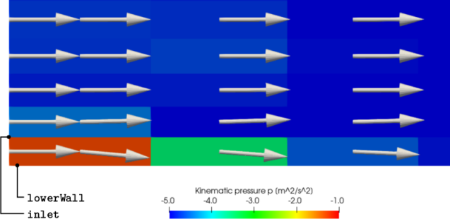
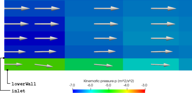
The velocity profile can be shown by returning to the Glyph module in the Pipeline Browser and making it visible. The profile can be illustrated by scaling the arrows by the the flow speed. In the Properties of the Glyph, scroll down to the Scale panel and set Scale Array to U, with Scale By Magnitude and a Scale Factor of 8e-05. The vectors are assigned a Solid Color of white.
The figure shows the inlet region adjacent to the lower wall boundary. At the left of the image, the vectors show a uniform profile. Shear at the wall causes the flow to decelerate, starting in the near-wall cell. The deceleration causes an increase in pressure, which produces a driving gradient that redirects the flow slightly away from the wall, to obey mass conservation.
In order to reduce the pressure increase, the boundary condition can be modified so that the inlet velocity is no longer uniform. A flowRateInletVelocity boundary condition is a general boundary condition for U, specifying flow at an inlet. Documentation for this boundary condition can be viewed using the foamInfo script, a general tool which provides documentation for applications, models and tools in OpenFOAM. It is run for the flowRateInletVelocity boundary condition as follows (noting that the name can sometimes be abbreviated for simplicity, here flowRateInlet, rather than flowRateInletVelocity).
foamInfo flowRateInlet
The documentation explains that the flowRateInletVelocity condition can specify the flow by a massFlowRate, volumetricFlowRate or meanVelocity. The user should open the 0/U in their editor and locate the boundary field entry for the inlet patch. The condition with a meanVelocity can then be applied by changing the inlet sub-dictionary as follows:
inlet
{
type flowRateInletVelocity; // modify
meanVelocity 10; // insert
value uniform (10 0 0); // leave
}
After saving the 0/U file, the user can re-run the simulation to check first that the flowRateInletVelocity emulates the original fixedValue condition. The controlDict file specifies that case starts from time 0 and it will overwrite previous results in time directories. The user can test the new condition simply by re-running the foamRun solver.
foamRun
The user should now modify the flowRateInletVelocity condition in the 0/U file by including a profile for the velocity. The documentation highlights two customised profile function, turbulentBL and laminarBL, which provide power-law and quadtratic profiles for fully-developed turbulent and laminar boundary layers, respectively. In this example, add the turbulentBL profile to the boundary condition as follows:
inlet
{
type flowRateInletVelocity;
meanVelocity 10;
profile turbulentBL; // add
value uniform (10 0 0);
}
The foamListTimes utility provides a quick, simple way to delete solution time directories, i.e. retaining the 0 directory. First run foamListTimes in the terminal as follows:
foamListTimes
foamListTimes -rm
The change in output times may create confusion for ParaView, causing it to query times in the time selector with (?) symbols. The selector entries can be rebuilt by reverting to time 0 or clicking Cache Mesh and Apply. The user can then select the last time in the sequence (277).
The velocity profile and pressure are updated as
shown in Figure 2.11
. For
pressure, the custom range is moved to  . The velocity is no
longer uniform at the inlet, but forms a profile according to the
turbulentBL function. The
velocity magnitude at the face adjacent to the lower wall is
significantly reduced from previously so the deceleration due to
shear is also reduced in the near-wall cell. The pressure difference
between the left corner and surrounding cells is consequently not
as high, approximately +2
. The velocity is no
longer uniform at the inlet, but forms a profile according to the
turbulentBL function. The
velocity magnitude at the face adjacent to the lower wall is
significantly reduced from previously so the deceleration due to
shear is also reduced in the near-wall cell. The pressure difference
between the left corner and surrounding cells is consequently not
as high, approximately +2  (from -7 to -5)
compared to +4 (from -5 to -1) previously.
(from -7 to -5)
compared to +4 (from -5 to -1) previously.
2.1.18 Turbulence model
The backward step case is set up to allow users
to try out different turbulence models quickly. There is comment in
the momentumTransport file in
the constant directory,
listing different turbulence models tested on this case. Some of the
models solve equations for fields other than  and
and  , e.g.
  (omega). To minimise the work when changing
models, files for these other fields are already included in the
0 directory. Similarly,
entries for schemes and solvers for these fields are included in the
fvSchemes and fvSolution files, respectively (in the
system directory).
(omega). To minimise the work when changing
models, files for these other fields are already included in the
0 directory. Similarly,
entries for schemes and solvers for these fields are included in the
fvSchemes and fvSolution files, respectively (in the
system directory).
The user should open the momentumTransport file in their editor to
change the turbulence model. They can change the model to
realizable  –
– by the following setting.
model realizableKE;
foamListTimes -rm
foamRun
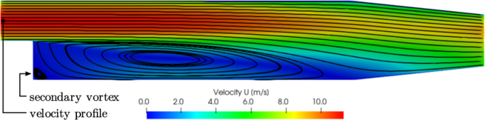
The realizable – model is less diffusive
that the standard
model is less diffusive
that the standard  – model. It captures a secondary vortex at the base of
the step which is approximately half the step height. The
recirculation region is also longer, with reattachment occurring at
the point the lower wall begins to taper towards the outlet.
– model. It captures a secondary vortex at the base of
the step which is approximately half the step height. The
recirculation region is also longer, with reattachment occurring at
the point the lower wall begins to taper towards the outlet.
 model.
The user can also test other turbulence models.
The  –
– SST model is a popular choice in industrial CFD which can
be selected by the following setting in the momentumTransport file.
SST model is a popular choice in industrial CFD which can
be selected by the following setting in the momentumTransport file.
model kOmegaSST;
It requires initialisation of specific turbulent
dissipation rate  . Item can be calculated similarly to
  in
Equation 2.3
using
in
Equation 2.3
using  as follows:
 |
(2.4) |
 = 2.54 mm as before,
  In the 0/omega file, 440.2 is used both for the initial
internalField and the inlet
value.
In the 0/omega file, 440.2 is used both for the initial
internalField and the inlet
value.
The simulation can now be re-run using this model by deleting the solution time directories and executing foamRun as before. The solver does not terminate early by converging to within the tolerances specified in the residualControl sub-dictionary of the fvSolution file. Instead, it terminates at 2000 iterations, the endTime specified in the controlDict file.
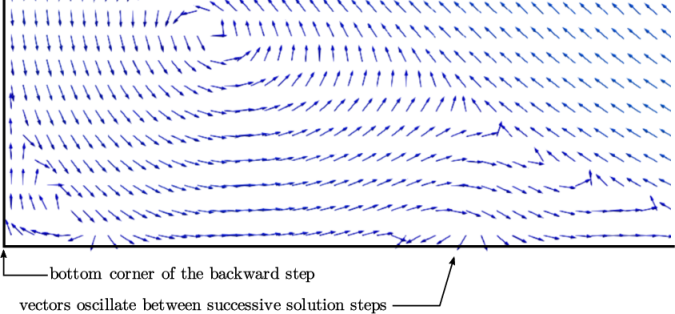
The results with the  –
– SST model show a larger
secondary vortex at the base of the step. The vortex does not
stabilise to a steady-state, but instead oscillates a small amount
over successive solution steps. The oscillations can be seen by
examining the velocity vectors at different solution steps,
e.g. 1000, 1100, 1200, etc. Figure 2.13
shows the extent of the secondary vortex and indicates where
vectors oscillate around the reattachment point of the vortex.
SST model show a larger
secondary vortex at the base of the step. The vortex does not
stabilise to a steady-state, but instead oscillates a small amount
over successive solution steps. The oscillations can be seen by
examining the velocity vectors at different solution steps,
e.g. 1000, 1100, 1200, etc. Figure 2.13
shows the extent of the secondary vortex and indicates where
vectors oscillate around the reattachment point of the vortex.
 –
– SST model.
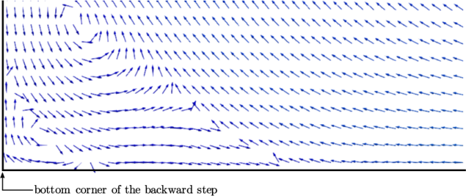
 –
– SST model with limiting
on
SST model with limiting
on The secondary vortex can be stabilised by a change to the numerical scheme for momentum advection. The user should open the fvSchemes file from the system directory. The discretisation of the advection terms is specified by the keyword entries of the form “div(phi,…)” in the divSchemes sub-dictionary. Momentum advection uses the linearUpwind scheme as shown below.
div(phi,U) bounded Gauss linearUpwind grad(U);
In order to stabilise the secondary vortex, the cellLimited scheme can be applied specifically to the discretisation of the velocity gradient grad(U). The syntax is shown below.
gradSchemes
{
default Gauss linear;
grad(U) cellLimited Gauss linear 1;
}